suppressMessages({
  library(ggplot2)
  library(dplyr)
  library(skimr)
  library(shiny)
  library(DT)
  library(here)
  library(rsconnect)
  library(tidymodels)
  library(tidyverse)
  library(yardstick)
  library(MASS)
  library(broom)
  library(purrr)
})fitting-exercise
`
Load dataset
dataset found at https://github.com/metrumresearchgroup/BayesPBPK-tutorial.git
file_path_mav = here("fitting-exercise", "data", "Mavoglurant_A2121_nmpk.csv")
mav = read.csv(file_path_mav)
DV is the outcome variable
Plot graph DV as a function of Time by DOSE and ID
# Create a ggplot object using the 'mav' data
ggplot(mav, aes(x = TIME, y = DV, group = ID, color = as.factor(DOSE))) +
  geom_line() +
  geom_point() +
  theme_minimal() +
  labs(title = "DV as a function of Time by DOSE and ID",
       x = "Time",
       y = "DV",
       color = "Dose")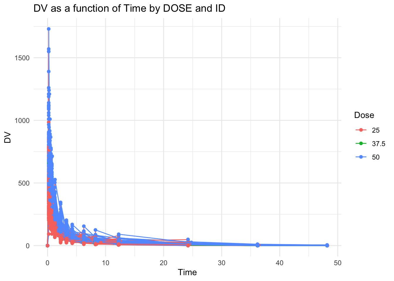
Showing all doses on one graph make it difficult to read
Try creating 1 plot for each dose
ggplot(mav, aes(x = TIME, y = DV, group = ID, color = as.factor(DOSE))) +
  geom_line() +
  geom_point() +
  theme_minimal() +
  labs(title = "DV as a function of Time by DOSE and ID",
       x = "Time",
       y = "DV",
       color = "Dose") +
  facet_grid(~DOSE, scales = "fixed")  # Adjusted scales to "fixed" so that they share the same y axis scale.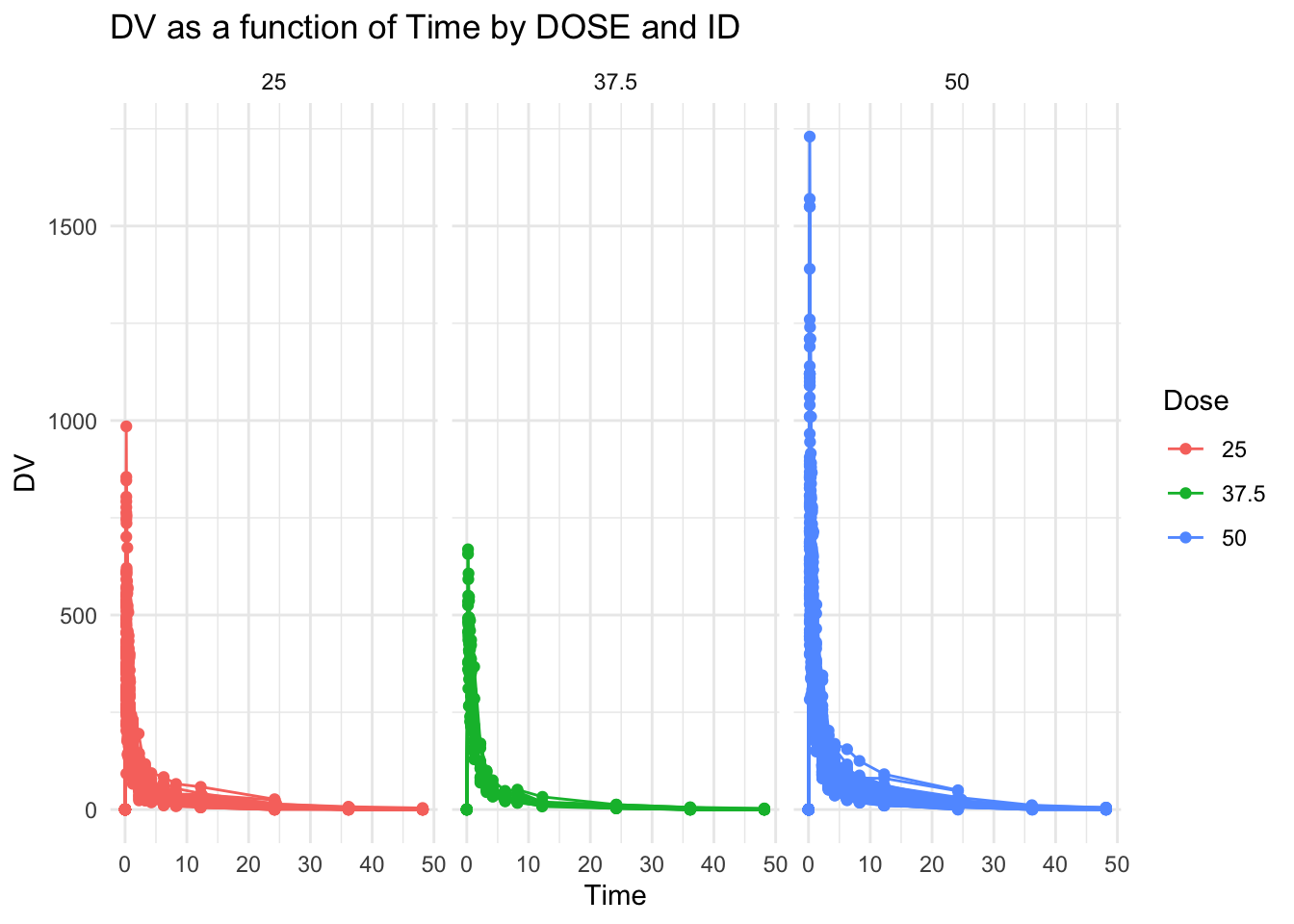
Keep only records where OCC=1
mav_occ_1 = mav %>%
    filter(OCC == 1)

#check to make sure filter worked as expected
unique(mav_occ_1$OCC)
[1] 1Filter and join the dataset
One data frame where observations where TIME = 0 are excluded, then sum DV for each ID to create a new variable, Y
One data frame that keeps only records where TIME == 0
Rationale: Initial measurements (TIME == 0) often represent baseline or pre-treatment values. Excluding these when summing DV allows for the calculation of total change or exposure post-baseline, which can be critical for assessing the effect or impact of an intervention.
# exclude observations where TIME = 0
# then sum DV for each ID to create new variable, Y
mav_dv_sum = mav_occ_1 %>%
  filter(TIME != 0) %>%
  group_by(ID) %>%
  summarize(Y = sum(DV, na.rm = TRUE))

#check dimension
dim(mav_dv_sum)
[1] 120 2# Keep only records where TIME == 0
mav_time0 = mav_occ_1 %>%
filter(TIME == 0) %>%
distinct(ID, .keep_all = TRUE)
#join the two data frames
mav_joined = left_join(mav_dv_sum, mav_time0, by = "ID")
#Check the dimension to ensure it is 120x18
dim(mav_joined)[1] 120 18Convert SEX, RACE, and DOSE to factor variables and keep the variables Y, DOSE, AGE, SEX, RACE, WT, HT
#This code transforms SEX, RACE, and DOSE into categorical variables for analysis and selects a specific set of variables, streamlining the dataset for focused statistical modeling or data exploration involving these key demographic and treatment attributes.
library(dplyr)
mav_clean <- mav_joined %>%
  mutate(SEX = as.factor(SEX), RACE = as.factor(RACE), DOSE = as.factor(DOSE)) %>%
  dplyr::select(Y, DOSE, AGE, SEX, RACE, WT, HT)

# Define the path using here() to the desired folder
# This will be used in Ex 11
file_path_ex11 <- here("ml-models-exercise", "mav_clean_ex11.rds")

saveRDS(mav_clean, file = file_path_ex11)


# Checking the dimensions
dim(mav_clean)
[1] 120 7Create BMI variable and a categorical variable for age
Convert them to factors
BMI = weight in kilograms / (height in meters)^2
#Calculate BMI and assign categories based on value
mav_clean <- mav_clean %>%
  mutate(
    bmi = WT / (HT^2),
    BMI_Category = case_when(
      bmi < 18.5 ~ "Underweight",
      bmi >= 18.5 & bmi < 25 ~ "Normal",
      bmi >= 25 & bmi < 30 ~ "Overweight",
      bmi >= 30 ~ "Obese",
      TRUE ~ "Unknown"  # Handles any missing or NA values
    )
  ) %>%
  mutate(BMI_Category = factor(BMI_Category)) #convert to factor

#Create categorical age variable
mav_clean <- mav_clean %>%
  mutate(Age_Group = cut(AGE,
                         breaks = c(-Inf, 18, 30, 40, 50, 60, Inf),
                         labels = c("<=18", "19-30", "31-40", "41-50", "51-60", ">60"),
                         right = FALSE)) %>%
    mutate(Age_Group = factor(Age_Group)) #convert to factor

# saving RDS for later use
#saveRDS(mav_clean, file = "/path")

#examine structure
str(mav_clean)
tibble [120 × 10] (S3: tbl_df/tbl/data.frame)
$ Y : num [1:120] 2691 2639 2150 1789 3126 ...
$ DOSE : Factor w/ 3 levels "25","37.5","50": 1 1 1 1 1 1 1 1 1 1 ...
$ AGE : int [1:120] 42 24 31 46 41 27 23 20 23 28 ...
$ SEX : Factor w/ 2 levels "1","2": 1 1 1 2 2 1 1 1 1 1 ...
$ RACE : Factor w/ 4 levels "1","2","7","88": 2 2 1 1 2 2 1 4 2 1 ...
$ WT : num [1:120] 94.3 80.4 71.8 77.4 64.3 ...
$ HT : num [1:120] 1.77 1.76 1.81 1.65 1.56 ...
$ bmi : num [1:120] 30.1 26 21.9 28.4 26.4 ...
$ BMI_Category: Factor w/ 3 levels "Normal","Obese",..: 2 3 1 3 3 1 3 1 1 2 ...
$ Age_Group : Factor w/ 4 levels "19-30","31-40",..: 3 1 2 3 3 1 1 1 1 1 ...Create tables
Calculatec summary statistics (number of observations, mean, median, minimum, and maximum of variable Y) for different groups in the dataset mav_clean, based on SEX, BMI_Category, and Age_Group
Display these values in sortable tables
# Compute summary statistics for each factor variable
summary_sex <- mav_clean %>%
  group_by(SEX) %>%
    summarize(
    N = n(),
    Mean_Y = mean(Y, na.rm = TRUE),
    Median_Y = median(Y, na.rm = TRUE),
    Min_Y = min(Y, na.rm = TRUE),
    Max_Y = max(Y, na.rm = TRUE),
    .groups = 'drop'
  ) %>%
  mutate(across(c(Mean_Y, Median_Y, Min_Y, Max_Y), round, 2))
Warning: There was 1 warning in `mutate()`.
ℹ In argument: `across(c(Mean_Y, Median_Y, Min_Y, Max_Y), round, 2)`.
Caused by warning:
! The `...` argument of `across()` is deprecated as of dplyr 1.1.0.
Supply arguments directly to `.fns` through an anonymous function instead.
# Previously
across(a:b, mean, na.rm = TRUE)
# Now
across(a:b, \(x) mean(x, na.rm = TRUE))summary_BMI <- mav_clean %>%
group_by(BMI_Category) %>%
summarize(
N = n(),
Mean_Y = mean(Y, na.rm = TRUE),
Median_Y = median(Y, na.rm = TRUE),
Min_Y = min(Y, na.rm = TRUE),
Max_Y = max(Y, na.rm = TRUE),
.groups = 'drop'
) %>%
mutate(across(c(Mean_Y, Median_Y, Min_Y, Max_Y), round, 2))
summary_age <- mav_clean %>%
group_by(Age_Group) %>%
summarize(
N = n(),
Mean_Y = mean(Y, na.rm = TRUE),
Median_Y = median(Y, na.rm = TRUE),
Min_Y = min(Y, na.rm = TRUE),
Max_Y = max(Y, na.rm = TRUE),
.groups = 'drop'
) %>%
mutate(across(c(Mean_Y, Median_Y, Min_Y, Max_Y), round, 2))
# Display the tables
datatable(summary_sex, options = list(pageLength = 5), caption = 'Summary Statistics of Y by SEX')datatable(summary_BMI, options = list(pageLength = 5), caption = 'Summary Statistics of Y by BMI')datatable(summary_age, options = list(pageLength = 5), caption = 'Summary Statistics of Y by Age')Computes summary statistics (count, mean, median, minimum, and maximum) for variable Y, grouped by Age_Group and BMI_Category from the mav_clean dataset, and then displays the results in an sortable table
# Compute summary statistics for Y, stratified by both SEX and RACE
summary_stats_group <- mav_clean %>%
  group_by(Age_Group, BMI_Category) %>%
  summarize(
    N = n(),
    Mean_Y = mean(Y, na.rm = TRUE),
    Median_Y = median(Y, na.rm = TRUE),
    Min_Y = min(Y, na.rm = TRUE),
    Max_Y = max(Y, na.rm = TRUE),
    .groups = 'drop'
  ) %>%
  mutate(across(c(Mean_Y, Median_Y, Min_Y, Max_Y), round, 2))

# Display the table with DT::datatable for interactivity
datatable(summary_stats_group, options = list(pageLength = 10),
          caption = 'Summary Statistics of Y by Age and BMI Status')
This R code reorders the levels of the factor variable BMI_Category in the dataset mav_clean and then creates four different plots: a raincloud plot of Y by BMI_Category, a combines scatter and contour plot of Y by Weight, a raincloud plot of Y by DOSE, and a raincloud plot of Y by age category using the ggplot2 package in R
# Reorder the levels of BMI_Category
mav_clean$BMI_Category <- factor(mav_clean$BMI_Category,
                                  levels = c("Normal", "Overweight", "Obese"))

ggplot(mav_clean, aes(x = BMI_Category, y = Y)) +
  geom_violin(fill = "skyblue", alpha = 0.5) +  # Add violin plot with semi-transparent fill
  geom_boxplot(width = 0.1, fill = "white", color = "black", outlier.shape = NA) +  # Add transparent boxplot without outliers
  geom_point(position = position_jitter(width = 0.2), alpha = 0.5, size = 2) +  # Add jittered points for individual data
  labs(x = "BMI", y = "Y", title = "Raincloud Plot of Y by BMI")  # Add labels and title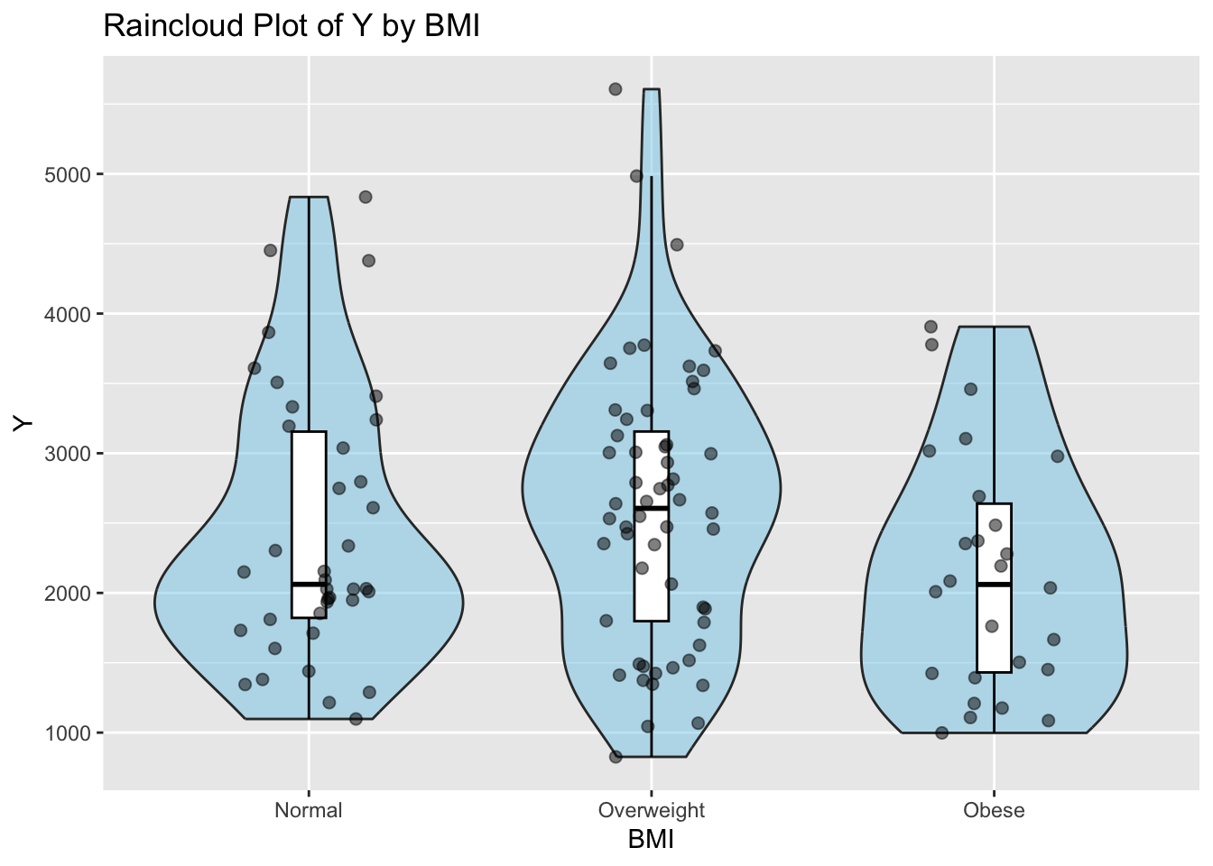
ggplot(mav_clean, aes(x = WT, y = Y)) +
  geom_point() +
  labs(x = "Weight (kg)", y = "Y", title = "Scatter Plot of Y by Weight")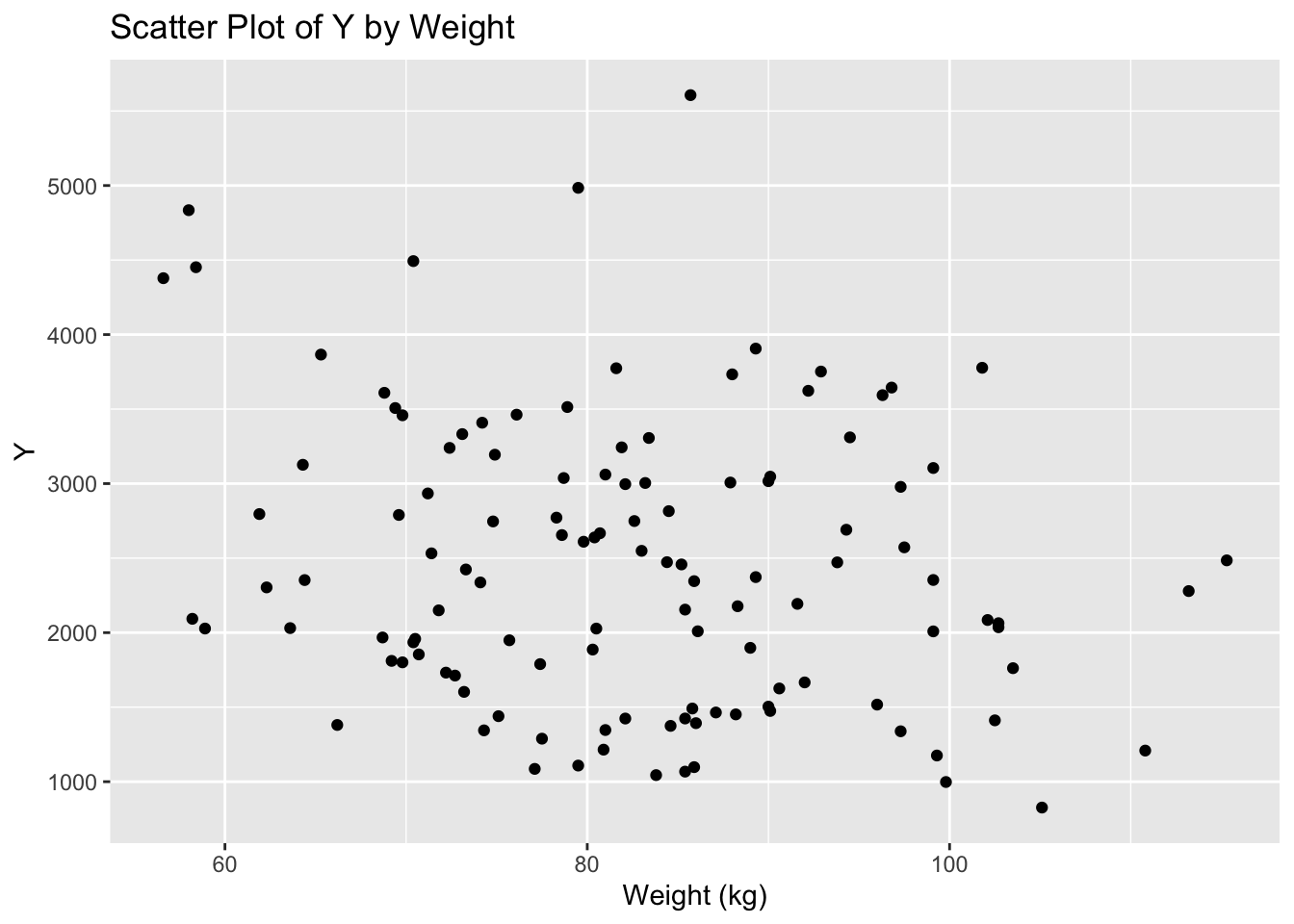
#Combined scatter and contour plot
#a contour plot displays the density of points
#in the form of contour lines, providing a two-dimensional representation of the data density.
ggplot(mav_clean, aes(x = WT, y = Y)) +
  stat_density_2d(aes(fill = after_stat(level)), geom = "polygon") +  # Create contour polygons
  geom_point() +  # Add scatter plot
  scale_fill_viridis_c() +  # Choose a color scale
  labs(x = "Weight (kg)", y = "Y", title = "Combined Scatter and Contour Plot of Y by Weight")  # Add labels and title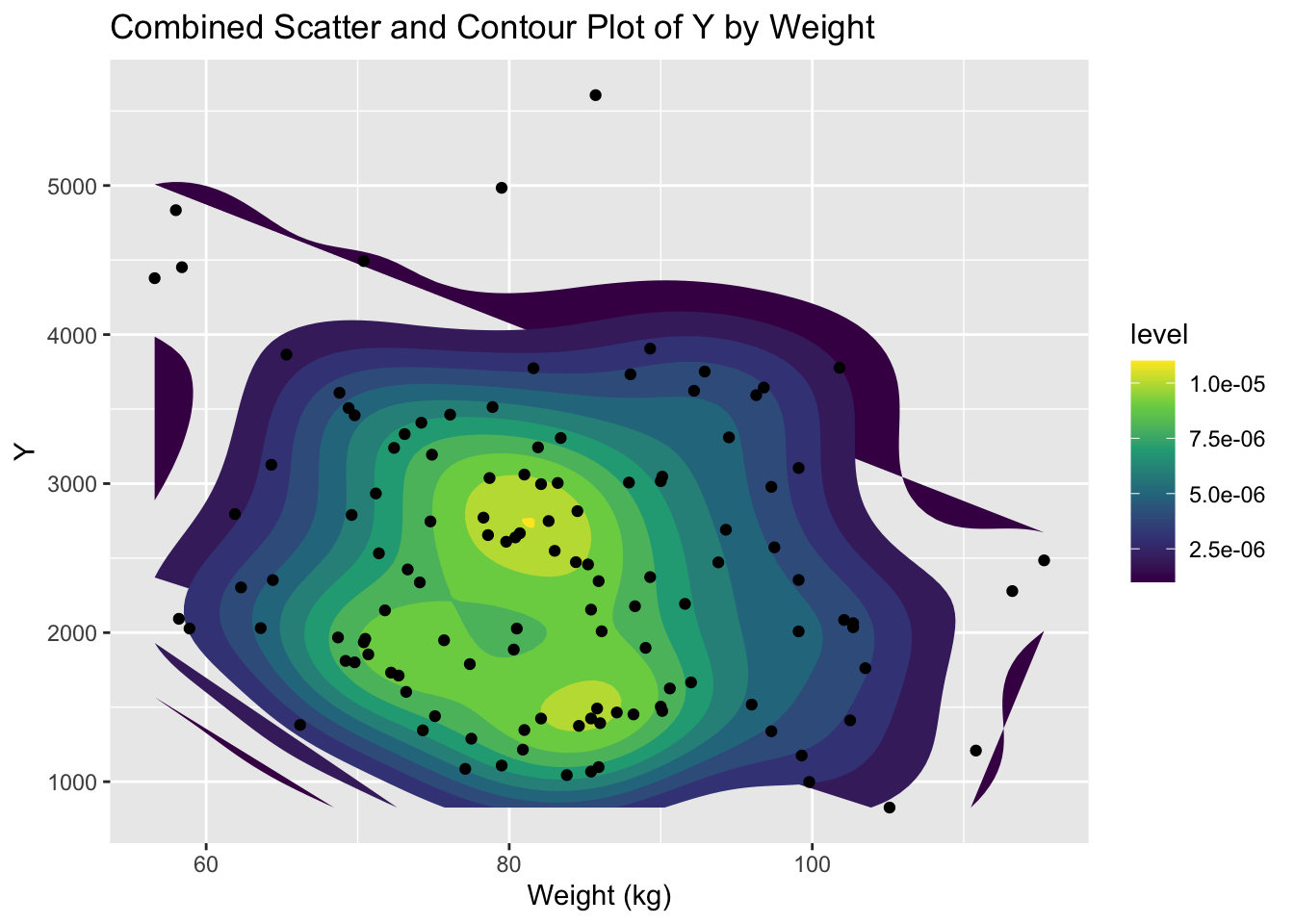
ggplot(mav_clean, aes(x = DOSE, y = Y)) +
  geom_violin(fill = "skyblue", alpha = 0.5) +  # Add violin plot with semi-transparent fill
  geom_boxplot(width = 0.1, fill = "white", color = "black", outlier.shape = NA) +  # Add transparent boxplot without outliers
  geom_point(position = position_jitter(width = 0.2), alpha = 0.5, size = 2) +  # Add jittered points for individual data
  labs(x = "DOSE", y = "Y", title = "Raincloud Plot of Y by Dose")  # Add labels and title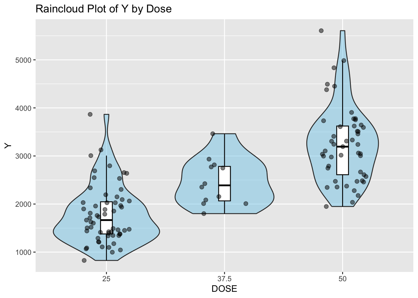
ggplot(mav_clean, aes(x = Age_Group, y = Y)) +
  geom_violin(fill = "skyblue", alpha = 0.5) +  # Add violin plot with semi-transparent fill
  geom_boxplot(width = 0.1, fill = "white", color = "black", outlier.shape = NA) +  # Add transparent boxplot without outliers
  geom_point(position = position_jitter(width = 0.2), alpha = 0.5, size = 2) +  # Add jittered points for individual data
  labs(x = "Age_Group", y = "Y", title = "Raincloud Plot of Y by Age")  # Add labels and title
Warning: Groups with fewer than two datapoints have been dropped.
ℹ Set `drop = FALSE` to consider such groups for position adjustment purposes.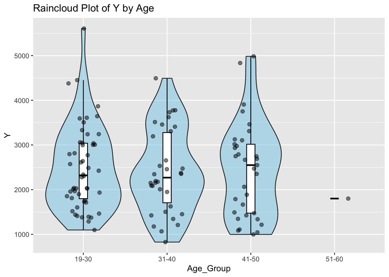
Create a grid of scatterplots for each pair of variables in subset_data (Y, bmi) and (HT, bmi), along with histograms for each variable on the diagonal and correlation coefficients in the upper triangle.
Weight and BMI are directly related. Using this as an example to show highly correlated pair
# Load the GGally library for pair plot visualization
library(GGally)
Registered S3 method overwritten by 'GGally':
method from
+.gg ggplot2# Subset the dataset to include only the variables Y and BMI
subset_Ybmi<- mav_clean[, c("Y", "bmi")]
# Using the pairs() function to create a matrix of scatterplots for Y and BMI
pairs(subset_Ybmi)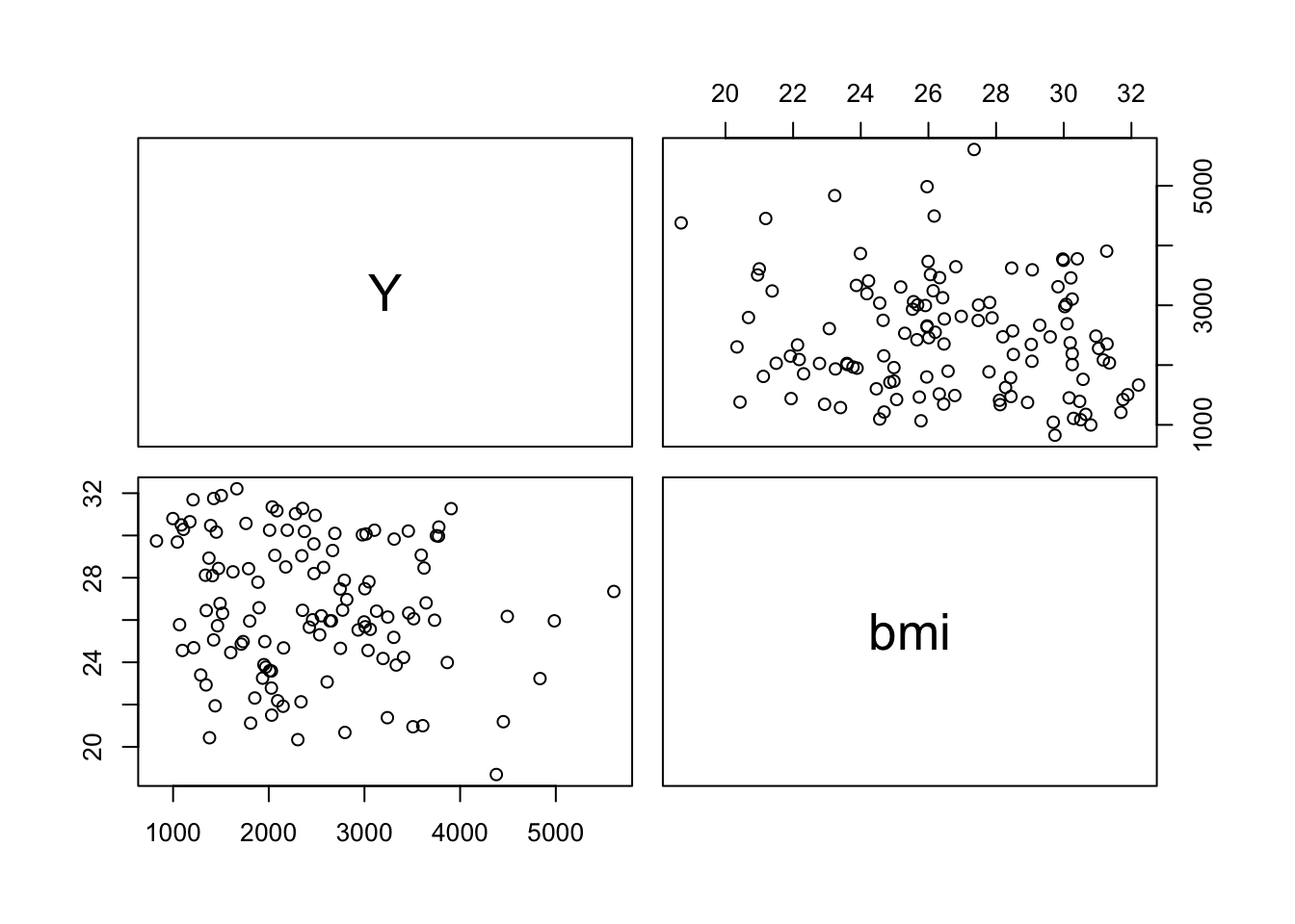
# Using the ggpairs() function to create a grid of scatterplots, histograms, and correlation coefficients for Y and BMI
ggpairs(subset_Ybmi)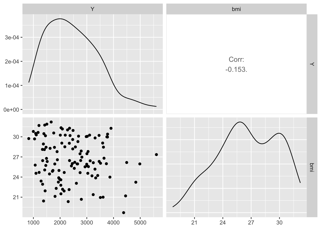
# Subset the dataset to include only the variables weight and BMI
subset_dataWTbmi <- mav_clean[, c("WT", "bmi")]

# Using the pairs() function to create a matrix of scatterplots for weight and BMI
pairs(subset_dataWTbmi)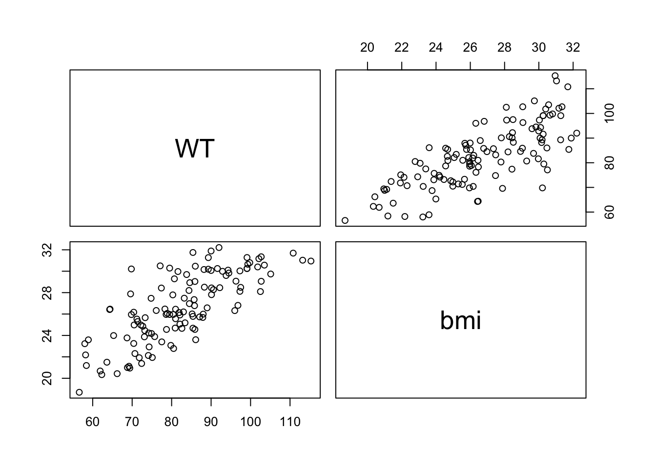
# Using the ggpairs() function to create a grid of scatterplots, histograms, and correlation coefficients for weight and BMI
ggpairs(subset_dataWTbmi)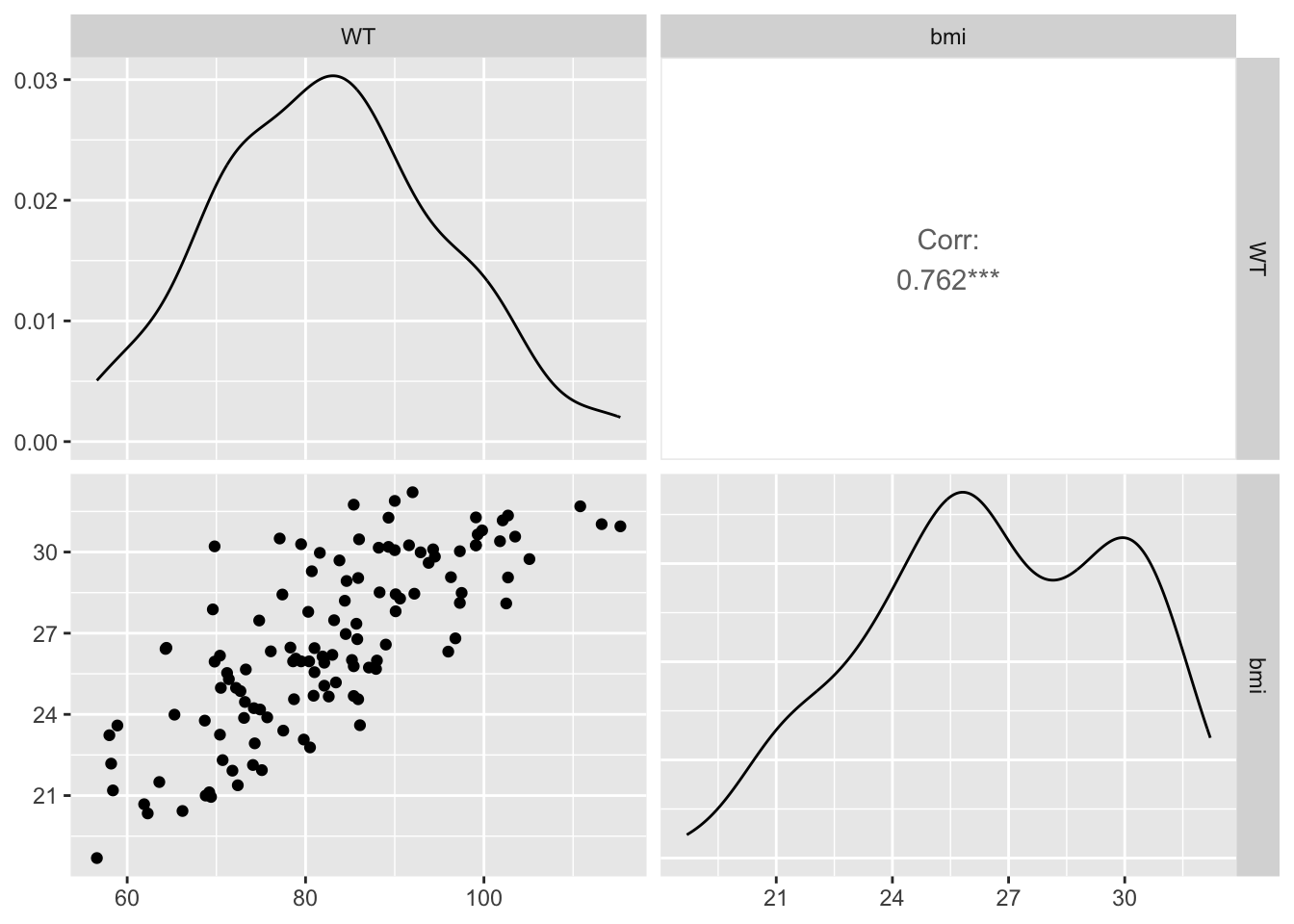
The BMI to Y shows a Corr. of -.0153. This suggests that there is weak inverse relationship between the two variables.
Model fitting
Fit a linear model to the continuous outcome (Y) using the main predictor of interest, DOSE
Fit a linear model to the continuous outcome (Y) using all predictors
Preprocess data
# Preprocess your data: convert 'DOSE' and 'BMI_Category' to factors
mav_clean <- mav_clean %>%
  mutate(
    DOSE = as.factor(DOSE),  # Convert DOSE to a factor
    BMI_Category = factor(BMI_Category, levels = c("Normal", "Overweight", "Obese"))  # Ensure BMI_Category has ordered levels
  )
The code defines a linear model specification using the ‘lm’ engine for regression analysis and prepares a 5-fold cross-validation with stratification by ‘Y’ to ensure balanced splits
Utilizing a 5-fold cross-validation with stratification by ‘Y’ helps ensure balanced splits within each fold, which is crucial for maintaining the representativeness of each subset during model evaluation, especially in the presence of class imbalance or uneven distribution of the target variable ‘Y’.
# Define the linear model specification using the 'lm' engine
linear_spec <- linear_reg() %>%
  set_engine("lm") %>%
  set_mode("regression")

# Prepare a 5-fold cross-validation, stratifying by 'Y' to ensure balanced splits
cv_folds <- vfold_cv(mav_clean, v = 5, strata = Y)
The code creates a workflow for a linear regression model using ‘DOSE’ as the predictor variable, fits the model across cross-validation folds, and collects evaluation metrics including Root Mean Squared Error (RMSE) and R-squared
# Create a workflow for the model using only DOSE as the predictor
workflow_dose <- workflow() %>%
  add_formula(Y ~ DOSE) %>%  # Define the model formula with DOSE
  add_model(linear_spec)  # Add the linear model specification

# Fit the model across the cross-validation folds and collect evaluation metrics (RMSE and R-squared)
results_dose <- fit_resamples(
  workflow_dose,
  cv_folds,
  metrics = metric_set(rmse, rsq)
)
This code creates a workflow for a linear regression model including all predictors (DOSE, AGE, and BMI_Category), fits the model across cross-validation folds, and collects evaluation metrics such as Root Mean Squared Error (RMSE) and R-squared.
# Workflow for the model including all predictors (DOSE, AGE, BMI_Category)
workflow_all <- workflow() %>%
  add_formula(Y ~ DOSE + AGE + BMI_Category) %>%  # Include all predictors in the formula
  add_model(linear_spec)  # Add the same linear model specification

# Fit this comprehensive model across the cross-validation folds and collect metrics
results_all <- fit_resamples(
  workflow_all,
  cv_folds,
  metrics = metric_set(rmse, rsq)
)
This series of steps allows for the comparison of evaluation metrics between the model with only ‘DOSE’ as the predictor and the model with all predictors (‘DOSE’, ‘AGE’, and ‘BMI_Category’). Additionally, it provides the range of values for the ‘Y’ variable in the dataset.
# Step 1: Collect metrics for the model with DOSE as the predictor
metrics_dose <- collect_metrics(results_dose)

# Step 2: Collect metrics for the model with all predictors
metrics_all <- collect_metrics(results_all)

# Step 3: Add a model identifier column to the metrics data frames AFTER collecting metrics
metrics_dose$model <- "DOSE Predictor"
metrics_all$model <- "All Predictors"

# Step 4: Combine metrics into a single data frame for comparison
combined_metrics <- bind_rows(metrics_dose, metrics_all)

# Step 5: Reorder the columns so that 'model' is the first column
reordered_metrics <- combined_metrics %>%
  dplyr::select(model, .metric, .estimator, mean, n, std_err, .config)

# Step 6: Print the reordered metrics
print(reordered_metrics)
# A tibble: 4 × 7
model .metric .estimator mean n std_err .config
<chr> <chr> <chr> <dbl> <int> <dbl> <chr>
1 DOSE Predictor rmse standard 659. 5 74.1 Preprocessor1_Model1
2 DOSE Predictor rsq standard 0.548 5 0.0574 Preprocessor1_Model1
3 All Predictors rmse standard 665. 5 75.4 Preprocessor1_Model1
4 All Predictors rsq standard 0.540 5 0.0652 Preprocessor1_Model1# Step 7: Print the range of 'Y' from the 'mav_clean' dataset
# Assuming 'mav_clean' is your dataset and it contains the variable 'Y'
y_range <- range(mav_clean$Y, na.rm = TRUE)
# Step 8: Print the range
print(y_range)[1] 826.43 5606.58Comparative Proportion: The error is a moderate proportion of the range (5606.58 - 826.43 = 4780.15). Specifically, it’s about 14% of the total range (666.90 / 4780.15 ≈ 0.14), suggesting that, on average, the model’s predictions might deviate from the actual values by around 14% of the total variability in Y.
Fit a logistic model to the categorical/binary outcome (SEX) using the main predictor of interest, which we’ll again assume here to be DOSE
Fit a logistic model to SEX using all predictors.
For both models, compute accuracy and ROC-AUC and print them
P(SEX = 1 | DOSE) = 1 / (1 + exp(-(intercept + coefficient * DOSE))
# Ensure SEX is a factor and DOSE is treated as a factor for logistic regression analysis
mav_clean_prepared <- mav_clean %>%
  mutate(
    SEX = as.factor(SEX),  # Convert SEX to a factor if it isn't already
    DOSE = as.factor(DOSE)  # Ensure DOSE is treated as a factor
  )

# Specify a logistic regression model using glm (Generalized Linear Model) as the engine
logistic_spec_dose <- logistic_reg() %>%
  set_engine("glm") %>%
  set_mode("classification")  # Set mode to classification for the binary outcome

# Prepare a 5-fold cross-validation object, stratifying by SEX to ensure balanced folds
cv_folds_sex <- vfold_cv(mav_clean_prepared, v = 5, strata = SEX)

# Create a workflow combining the logistic model specification with the SEX ~ DOSE formula
workflow_sex_dose <- workflow() %>%
  add_formula(SEX ~ DOSE) %>%  # Predicting SEX based on DOSE
  add_model(logistic_spec_dose)  # Add the logistic regression specification

# Fit the model across the cross-validation folds and calculate metrics
results_sex_dose_cv <- fit_resamples(
  workflow_sex_dose,
  cv_folds_sex,
  metrics = metric_set(roc_auc, accuracy)  # Focus on ROC AUC and accuracy for evaluation
)

# Collect and summarize the metrics from cross-validation
metrics_sex_dose <- collect_metrics(results_sex_dose_cv)

# Print the summarized metrics to assess model performance
print(metrics_sex_dose)
# A tibble: 2 × 6
.metric .estimator mean n std_err .config
<chr> <chr> <dbl> <int> <dbl> <chr>
1 accuracy binary 0.867 5 0.00681 Preprocessor1_Model1
2 roc_auc binary 0.565 5 0.0593 Preprocessor1_Model1Accuracy
Metric: Accuracy measures the proportion of true results (both true positives and true negatives) among the total number of cases examined. It’s a straightforward indicator of how often the model predicts the correct category.
Value: The mean accuracy across the 5 cross-validation folds is approximately 86.69%.
Interpretation: This suggests that, on average, the model correctly predicts the SEX category about 86.69% of the time across the different subsets of your data. A high accuracy indicates the model is generally effective at classifying the instances according to SEX.
ROC AUC (Area Under the Receiver Operating Characteristic Curve)
Metric: ROC AUC evaluates the model’s ability to discriminate between the classes at various threshold settings. The AUC (Area Under the Curve) ranges from 0 to 1, where 1 indicates perfect discrimination and 0.5 indicates no discrimination (equivalent to random guessing). Value: The mean ROC AUC across the 5 folds is approximately 0.553. Interpretation: This value is slightly above 0.5, indicating the model has a very limited ability to distinguish between the SEX categories beyond random chance. The ROC AUC being close to 0.5 suggests that, while the model is accurate in many of its predictions, this might be attributed to the distribution of classes in the dataset rather than the model’s discriminative power.
P(SEX = 1 | DOSE, AGE, BMI_Category) = 1 / (1 + exp(-(intercept + coefficient_DOSE * DOSE + coefficient_AGE * AGE + coefficient_BMI_Category * BMI_Category)))
# Preprocess the dataset: converting predictors to their appropriate formats
mav_clean_logistic_all <- mav_clean %>%
  mutate(
    BMI_Category = as.factor(BMI_Category),  # Ensure BMI_Category is a factor
    DOSE = as.factor(DOSE),  # Ensure DOSE is a factor
    AGE = as.numeric(AGE)  # Ensure AGE is numeric
  )

# Specify a logistic regression model using glm as the computational engine
logistic_spec_all <- logistic_reg() %>%
  set_engine("glm") %>%
  set_mode("classification")

# Prepare a 5-fold cross-validation, ensuring a balanced representation of SEX across folds
cv_folds_sex_all <- vfold_cv(mav_clean_logistic_all, v = 5, strata = SEX)

# Create a workflow that encapsulates the model specification and formula
workflow_sex_all <- workflow() %>%
  add_formula(SEX ~ BMI_Category + AGE + DOSE) %>%  # Use all predictors in the model formula
  add_model(logistic_spec_all)  # Add the logistic regression model specification

# Fit the model across the cross-validation folds and evaluate
results_sex_all_cv <- fit_resamples(
  workflow_sex_all,
  cv_folds_sex_all,
  metrics = metric_set(roc_auc, accuracy)  # Focus on ROC AUC and accuracy for evaluation
)
# Collect metrics from the cross-validation results
metrics_sex_all <- collect_metrics(results_sex_all_cv)

# Print the summarized metrics to understand model performance
print(metrics_sex_all)
# A tibble: 2 × 6
.metric .estimator mean n std_err .config
<chr> <chr> <dbl> <int> <dbl> <chr>
1 accuracy binary 0.825 5 0.0243 Preprocessor1_Model1
2 roc_auc binary 0.769 5 0.0316 Preprocessor1_Model1First Model (DOSE as the Predictor)
Accuracy: The mean accuracy is approximately 86.69%, indicating a high overall rate of correctly predicting SEX.
ROC AUC: The mean ROC AUC is approximately 0.553, suggesting the model’s ability to discriminate between the classes is only slightly better than random guessing.
Second Model (All Predictors: BMI_Category, AGE, DOSE)
Accuracy: The mean accuracy slightly decreases to approximately 84.26%. This indicates a slight reduction in the overall rate of correct predictions compared to the first model.
ROC AUC: The mean ROC AUC improves to approximately 0.627, indicating enhanced discriminative ability between the classes compared to the first model.
Interpretation
Accuracy vs. ROC AUC: While the first model achieves higher accuracy, its ROC AUC value is lower, suggesting it’s not as effective at distinguishing between the classes across different thresholds. The second model, despite a slight drop in accuracy, shows a notable improvement in ROC AUC, indicating better performance in class discrimination.
Model Comparison: The increase in ROC AUC for the second model suggests that including additional predictors (BMI_Category and AGE alongside DOSE) contributes to a more nuanced understanding and prediction of SEX, beyond what is achievable with DOSE alone. This indicates the importance of considering multiple factors in predictive modeling, especially for complex outcomes.
k-nearest neighbors (KNN) regression model
The model is trained and evaluated to predict the outcome variable ‘Y’ based on the predictor variable ‘DOSE’.
This process involves splitting the dataset into training and testing sets, converting the ‘DOSE’ variable to a factor, specifying the KNN model, fitting the model on the training data, making predictions on the testing set, calculating evaluation metrics (Root Mean Squared Error and R-squared), and printing the evaluation metrics for model assessment and comparison.
library(kknn)

# Splitting the data
set.seed(123)  # Ensure reproducibility
mav_data_split <- initial_split(mav_clean, prop = 0.75)  # 75% training, 25% testing
mav_train <- training(mav_data_split)  # Training data
mav_test <- testing(mav_data_split)  # Testing data

mav_train <- mav_train %>%
  mutate(DOSE = as.factor(DOSE))

mav_test <- mav_test %>%
  mutate(DOSE = as.factor(DOSE))

# KNN model specification
knn_spec <- nearest_neighbor(neighbors = 5) %>%
  set_engine("kknn") %>%
  set_mode("regression")

# Creating the workflow
knn_workflow <- workflow() %>%
  add_formula(Y ~ DOSE) %>%
  add_model(knn_spec)

# Fitting the model on training data
knn_fit <- knn_workflow %>%
  fit(data = mav_train)

# Making predictions on the testing set
knn_predictions <- predict(knn_fit, new_data = mav_test) %>%
  bind_cols(mav_test)

# Calculate RMSE and R-squared
knn_metrics <- knn_predictions %>%
  metrics(truth = Y, estimate = .pred) %>%
  filter(.metric %in% c("rmse", "rsq"))

# Print the evaluation metrics
print(knn_metrics)
# A tibble: 2 × 3
.metric .estimator .estimate
<chr> <chr> <dbl>
1 rmse standard 566.
2 rsq standard 0.648Model comparison
RMSE (Root Mean Squared Error):
KNN model: 565.72
“DOSE Predictor” model: 673.09
The RMSE of the KNN model (565.72) is lower than that of the “DOSE Predictor” model (673.09), indicating that, on average, the KNN model’s predictions are closer to the true values compared to the “DOSE Predictor” model.
R-squared (rsq):
KNN model: 0.648
“DOSE Predictor” model: 0.522
The R-squared value of the KNN model (0.648) is higher than that of the “DOSE Predictor” model (0.522), suggesting that the KNN model explains a higher proportion of the variance in the outcome variable compared to the “DOSE Predictor” model.
Overall, based on these metrics, the KNN model appears to perform better in terms of both accuracy (lower RMSE) and explanatory power (higher R-squared) compared to the “DOSE Predictor” model.
Exercise 10
Improving Models
Data prep
First we will set a random seed.
We will specify a value for a seed at the start, and then re-set the seed to this value before every operation that involves random numbers.
rngseed2 = 1234To pick up where we left off, let’s re-examine the dataset.
str(mav_clean)tibble [120 × 10] (S3: tbl_df/tbl/data.frame)
$ Y : num [1:120] 2691 2639 2150 1789 3126 ...
$ DOSE : Factor w/ 3 levels "25","37.5","50": 1 1 1 1 1 1 1 1 1 1 ...
$ AGE : int [1:120] 42 24 31 46 41 27 23 20 23 28 ...
$ SEX : Factor w/ 2 levels "1","2": 1 1 1 2 2 1 1 1 1 1 ...
$ RACE : Factor w/ 4 levels "1","2","7","88": 2 2 1 1 2 2 1 4 2 1 ...
$ WT : num [1:120] 94.3 80.4 71.8 77.4 64.3 ...
$ HT : num [1:120] 1.77 1.76 1.81 1.65 1.56 ...
$ bmi : num [1:120] 30.1 26 21.9 28.4 26.4 ...
$ BMI_Category: Factor w/ 3 levels "Normal","Overweight",..: 3 2 1 2 2 1 2 1 1 3 ...
$ Age_Group : Factor w/ 4 levels "19-30","31-40",..: 3 1 2 3 3 1 1 1 1 1 ...In the previous exercise, I added 3 new variable. For this exercise, I will remove them along with RACE so that only Y, DOSE, AGE, SEX, WT, HT remain.
The dataframe dimension should be 120X6
# Rename dataframe and remove 'RACE', 'bmi', 'BMI_Category', 'Age_Group' columns using dplyr
mav_ex10 <- mav_clean %>%
  dplyr::select(-RACE, -bmi, -BMI_Category, -Age_Group)
head(mav_ex10)
# A tibble: 6 × 6
Y DOSE AGE SEX WT HT
<dbl> <fct> <int> <fct> <dbl> <dbl>
1 2691. 25 42 1 94.3 1.77
2 2639. 25 24 1 80.4 1.76
3 2150. 25 31 1 71.8 1.81
4 1789. 25 46 2 77.4 1.65
5 3126. 25 41 2 64.3 1.56
6 2337. 25 27 1 74.1 1.83dim(mav_ex10)[1] 120 6Randomly split dataset into training (75%) and test (25%) frames using the seed defined above.
set.seed(rngseed2)

# Split the data into a 75% training set and a 25% test set
data_split_mav <- initial_split(mav_ex10, prop = 0.75)

# Extract the training and test sets
mav10_train_75pct <- training(data_split_mav)
mav10_test_25pct<- testing(data_split_mav)
Model Fitting
Use the tidymodels framework to fit two linear models to our continuous outcome of interest, (here, Y). The first model should only use DOSE as predictor, the second model should use all predictors. For both models, the metric to optimize should be RMSE
Model specification
# Define linear regression models for fitting: one with DOSE only, another with all predictors
# dose
model_spec_dose <- linear_reg() %>%
  set_engine("lm") %>%
  set_mode("regression")

# all predictors
model_spec_all <- linear_reg() %>%
  set_engine("lm") %>%
  set_mode("regression")
Creating and Preparing a Recipe
The process involves defining a data preprocessing recipe tailored to the training dataset and incorporating this unprepared recipe into model-specific workflows. Once the workflows are fitted to the training data, the recipe is automatically prepared and applied, seamlessly integrating data preprocessing with model training.
# Define two recipes: one for the DOSE-only model and another for the All-predictors model

# Define the recipe for the DOSE-only model without immediately preparing it
mav_recipe_dose <- recipe(Y ~ DOSE, data = mav10_train_75pct) %>%
  step_dummy(all_nominal(), -all_outcomes())

# Define the recipe for the All-predictors model without immediately preparing it
mav_recipe_all <- recipe(Y ~ ., data = mav10_train_75pct) %>%
  step_dummy(all_nominal(), -all_outcomes())

# Now, you can add these unprepared recipes to the workflows
workflow_dose <- workflow() %>%
  add_model(model_spec_dose) %>%
  add_recipe(mav_recipe_dose)

workflow_all <- workflow() %>%
  add_model(model_spec_all) %>%
  add_recipe(mav_recipe_all)

# Fit the workflows to the training data
fit_dose <- fit(workflow_dose, data = mav10_train_75pct)
fit_all <- fit(workflow_all, data = mav10_train_75pct)
Making Predictions and Calculating RMSE #### This code segment generates predictions using two different models (fit_dose and fit_all) on a testing dataset (mav10_train_75pct), then computes the Root Mean Squared Error (RMSE) for each model’s predictions compared to the true values (Y).
# Make predictions on the testing set and calculate RMSE for each model
preds_dose <- predict(fit_dose, new_data = mav10_train_75pct) %>%
  bind_cols(mav10_train_75pct)
preds_all <- predict(fit_all, new_data = mav10_train_75pct) %>%
  bind_cols(mav10_train_75pct)
rmse_dose <- rmse(preds_dose, truth = Y, estimate = .pred)
rmse_all <- rmse(preds_all, truth = Y, estimate = .pred)
Calculating RMSE and Model Comparison
This code block manually computes the Root Mean Squared Error (RMSE) for three different models: the ‘DOSE’ model, the ‘All Predictors’ model, and a Null model. It then prints the RMSE values to compare the performance of each model.
# Manually calculate the mean of 'Y' from the training set for the null model
mean_y <- mean(mav10_train_75pct$Y, na.rm = TRUE)
null_predictions <- rep(mean_y, nrow(mav10_train_75pct))
null_rmse <- sqrt(mean((mav10_train_75pct$Y - null_predictions)^2))

# Print RMSE values to compare model performances
cat("RMSE for DOSE model:", rmse_dose$.estimate, "\n")
RMSE for DOSE model: 702.7909 cat("RMSE for All Predictors model:", rmse_all$.estimate, "\n")RMSE for All Predictors model: 627.2724 cat("RMSE for Null model (manual):", null_rmse, "\n")RMSE for Null model (manual): 948.3526 #Model performance assessment 2 ## Cross validation (CV) ### Set seed
#use the same seed as the previous section 1234
set.seed(rngseed2)  # Ensuring reproducibility
# Set the seed for reproducibility
set.seed(rngseed2)
# Define the 10-fold cross-validation folds
cv_folds10 <- vfold_cv(mav10_train_75pct, v = 10)
# Define the model specifications
model_spec_dose <- linear_reg() %>%
set_engine("lm") %>%
set_mode("regression")
model_spec_all <- linear_reg() %>%
set_engine("lm") %>%
set_mode("regression")
# Define workflows
workflow_dose <- workflow() %>%
add_model(model_spec_dose) %>%
add_formula(Y ~ DOSE)
workflow_all <- workflow() %>%
add_model(model_spec_all) %>%
add_formula(Y ~ .)
# Perform cross-validation for the DOSE-only model
cv_results_dose <- fit_resamples(
workflow_dose,
cv_folds10,
metrics = metric_set(rmse)
)
# Perform cross-validation for the All-predictor model
cv_results_all <- fit_resamples(
workflow_all,
cv_folds10,
metrics = metric_set(rmse)
)
# cv_results_dose and cv_results_all contain the cross-validation results
# Extract and average RMSE for the DOSE-only model
cv_summary_dose <- cv_results_dose %>%
collect_metrics() %>%
filter(.metric == "rmse") %>%
summarize(mean_rmse_cv = mean(mean, na.rm = TRUE)) %>%
pull(mean_rmse_cv)
# Extract and average RMSE for the All-predictors model
cv_summary_all <- cv_results_all %>%
collect_metrics() %>%
filter(.metric == "rmse") %>%
summarize(mean_rmse_cv = mean(mean, na.rm = TRUE)) %>%
pull(mean_rmse_cv)
# Assuming cv_results_dose and cv_results_all contain the cross-validation results
# Extract and average RMSE for the DOSE-only model
cv_summary_dose <- cv_results_dose %>%
collect_metrics() %>%
filter(.metric == "rmse") %>%
summarize(mean_rmse_cv = mean(mean, na.rm = TRUE)) %>%
pull(mean_rmse_cv)
# Extract and average RMSE for the All-predictors model
cv_summary_all <- cv_results_all %>%
collect_metrics() %>%
filter(.metric == "rmse") %>%
summarize(mean_rmse_cv = mean(mean, na.rm = TRUE)) %>%
pull(mean_rmse_cv)
library(dplyr)
# Summarize RMSE for DOSE-only model
summary_dose <- cv_results_dose %>% collect_metrics()
# Summarize RMSE for All-predictor model
summary_all <- cv_results_all %>% collect_metrics()
# Combine summaries into a single table
combined_summary <- bind_rows(
data.frame(Model = "DOSE-only", summary_dose),
data.frame(Model = "All-predictor", summary_all)
)
# Print the combined summary
print(combined_summary) Model .metric .estimator mean n std_err .config
1 DOSE-only rmse standard 696.7098 10 68.09511 Preprocessor1_Model1
2 All-predictor rmse standard 652.7739 10 63.59876 Preprocessor1_Model1Interpreting the results
Dose only model
For the DOSE-only model, the RMSE obtained through cross-validation is slightly lower than the initial RMSE. This indicates that the model is quite stable and generalizes well to unseen data. The slight improvement in RMSE suggests that the initial evaluation might have slightly overestimated the model’s error, and the model actually performs a bit better on average across different subsets of the data.
All predictor model
In contrast, for the All-predictors model, the CV RMSE is higher than the initial RMSE. This could indicate that the model, when evaluated on the training set, might have been slightly overfitting to that specific data. When the model is assessed through cross-validation, which involves training and evaluating the model on multiple subsets of the data, the average error increases. This suggests that the model’s predictions are not as consistent across different subsets of data, highlighting a potential overfitting issue where the model learns specific patterns in the training set that don’t generalize as well to unseen data.
Null model
The Null Model, serving as a baseline, simply predicts the mean outcome for all observations without using any predictors. There’s no variation in its predictions, so cross-validation does not apply. The RMSE here serves to underscore the baseline level of error when no predictive modeling is attempted.
# Set new seed for reproducibility
set.seed(4444)


# Split the data into a 75% training set and a 25% test set
data_split_mav_new <- initial_split(mav_ex10, prop = 0.75)

# Extract the training and test sets
mav10_train_75pct_new <- training(data_split_mav)
mav10_test_25pct_new <- testing(data_split_mav)

# Define the 10-fold cross-validation folds
cv_folds10_new <- vfold_cv(mav10_train_75pct_new, v = 10)  # Assuming mav10_train_75pct_new is the new dataframe

# Define the model specifications
model_spec_dose_new <- linear_reg() %>%
  set_engine("lm") %>%
  set_mode("regression")

model_spec_all_new <- linear_reg() %>%
  set_engine("lm") %>%
  set_mode("regression")

# Define workflows
workflow_dose_new <- workflow() %>%
  add_model(model_spec_dose_new) %>%
  add_formula(Y ~ DOSE)

workflow_all_new <- workflow() %>%
  add_model(model_spec_all_new) %>%
  add_formula(Y ~ .)

# Perform cross-validation for the DOSE-only model
cv_results_dose_new <- fit_resamples(
  workflow_dose_new,
  cv_folds10_new,
  metrics = metric_set(rmse)
)

# Perform cross-validation for the All-predictor model
cv_results_all_new <- fit_resamples(
  workflow_all_new,
  cv_folds10_new,
  metrics = metric_set(rmse)
)

# Extract and average RMSE for the DOSE-only model
cv_summary_dose_new <- cv_results_dose_new %>%
  collect_metrics() %>%
  filter(.metric == "rmse") %>%
  summarize(mean_rmse_cv = mean(mean, na.rm = TRUE)) %>%
  pull(mean_rmse_cv)

# Extract and average RMSE for the All-predictors model
cv_summary_all_new <- cv_results_all_new %>%
  collect_metrics() %>%
  filter(.metric == "rmse") %>%
  summarize(mean_rmse_cv = mean(mean, na.rm = TRUE)) %>%
  pull(mean_rmse_cv)

# Summarize RMSE for DOSE-only model
summary_dose_new <- cv_results_dose_new %>% collect_metrics()

# Summarize RMSE for All-predictor model
summary_all_new <- cv_results_all_new %>% collect_metrics()

# Combine summaries into a single table
combined_summary_new <- bind_rows(
  data.frame(Model = "DOSE-only", summary_dose_new),
  data.frame(Model = "All-predictor", summary_all_new)
)

# Print the combined summary
print(combined_summary_new)
Model .metric .estimator mean n std_err .config
1 DOSE-only rmse standard 712.7537 10 64.50994 Preprocessor1_Model1
2 All-predictor rmse standard 646.3119 10 69.04694 Preprocessor1_Model1# Print RMSE values to compare model performances
cat("RMSE for DOSE model:", rmse_dose$.estimate, "\n")RMSE for DOSE model: 702.7909 cat("RMSE for All Predictors model:", rmse_all$.estimate, "\n")RMSE for All Predictors model: 627.2724 cat("RMSE for Null model (manual):", null_rmse, "\n")RMSE for Null model (manual): 948.3526 When a different random seed was used, the RMSE directions changed. For Dose-Only the mean RMSE went up to 712. This suggests that using the randomizationm from this seed, subsets are not as consistent than in the seed1234.
On the other hand, the RMSE for the all predictors CV model improved slightly. This suggests that model based on this randomization is stabler and generalizes well to unseen data.
This section was added by Arlyn Santiago
First I am going to plot the predicted values from all three models against the observed values of the training data.
# Assuming mav10_train_75pct is your training data and 'Y' is the outcome variable
# Assuming preds_dose$.pred, preds_all$.pred are your predictions from the dose and full model respectively
# Assuming mean_y is the mean of the observed outcomes used for the null model predictions

# Extract the observed Y values from the training data
observed_values <- mav10_train_75pct$Y

# Prepare a dataframe for the DOSE model predictions
preds_dose_df <- data.frame(Observed = observed_values, Predicted = preds_dose$.pred, Model = "Dose Model")

# Prepare a dataframe for the All Predictors model predictions
preds_all_df <- data.frame(Observed = observed_values, Predicted = preds_all$.pred, Model = "Full Model")

# Prepare a dataframe for the Null model predictions
null_preds_df <- data.frame(Observed = observed_values, Predicted = rep(mean_y, length(observed_values)), Model = "Null Model")

# Combine all predictions into a single data frame
all_preds_df <- bind_rows(preds_dose_df, preds_all_df, null_preds_df)

# Now, plot using ggplot2
ggplot(all_preds_df, aes(x = Observed, y = Predicted, color = Model)) +
  geom_point() +
  geom_abline(intercept = 0, slope = 1, linetype = "dashed", color = "black") +
  scale_color_manual(values = c("Dose Model" = "orchid", "Full Model" = "darkorange3", "Null Model" = "blue")) +
  scale_x_continuous(limits = c(0, 5000)) +
  scale_y_continuous(limits = c(0, 5000)) +
  labs(x = "Observed Values", y = "Predicted Values", title = "Observed vs. Predicted Values by Model") +
  theme_minimal()
Warning: Removed 3 rows containing missing values or values outside the scale range
(`geom_point()`).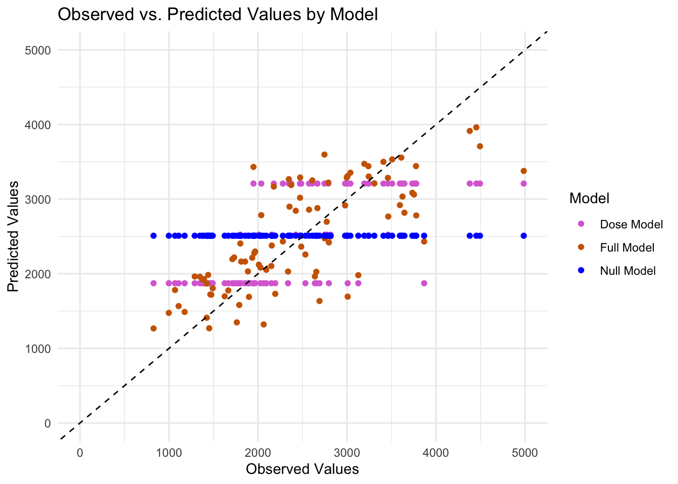
The predictions from Null model is a horizontal line, signifying that there is a single value which is the mean of the outcome variable. I decided to plot the predicted values against the residuals for the comprehensive model to further understand any relationship or patterns that can be found.
I computed the residuals and then generated the plot.
# Recalculate residuals using the correct column name
preds_all_df$residuals <- preds_all_df$Observed - preds_all_df$Predicted

# Find the maximum absolute residual to set the y-axis limits symmetrically
max_abs_residual <- max(abs(preds_all_df$residuals), na.rm = TRUE)

# Plot predicted vs residuals for the full model using the correct column names
ggplot(preds_all_df, aes(x = Predicted, y = residuals)) +
  geom_point(color = "tomato") +
  geom_hline(yintercept = 0, linetype = "dashed", color = "navy") +
  scale_y_continuous(limits = c(-max_abs_residual, max_abs_residual)) +
  labs(x = "Predicted Values", y = "Residuals", title = "Predicted vs. Residuals for the Full Model") +
  theme_minimal()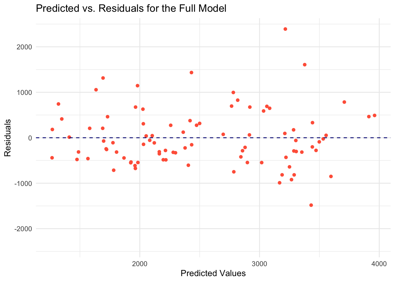
The model is not capturing some of the data. However, there are residuals grouped horizontally around 0.
Using the Bootstrap Method to test for Model Uncertainty
library(tidymodels)
library(purrr) # For the map function

# Set the random seed for reproducibility
set.seed(rngseed2) # Make sure rngseed2 is defined

# Create 100 bootstrap samples of the training data
boot_samples <- bootstraps(mav10_train_75pct, times = 100)

# Use the 'workflow_all' to fit the model to each of the bootstrap samples
# and make predictions on the original training data
predictions_list <- boot_samples$splits %>%
  map(.f = ~{
    # Extract the analysis (training) set from the current bootstrap sample
    boot_data <- analysis(.x)

    # Fit the workflow to the bootstrap sample. Assuming 'workflow_all' includes your model and preprocessing steps
    fitted_workflow <- fit(workflow_all, data = boot_data)

    # Make predictions on the original training data using the fitted workflow
    predict(fitted_workflow, new_data = mav10_train_75pct)$.pred
  })
# Check the length of the predictions list
# it should be 100
length(predictions_list)
[1] 100# Step 1: Convert the list of prediction vectors into a matrix with bootstrap samples as columns
bootstrap_predictions_matrix <- do.call(cbind, predictions_list)
# Ensure that the matrix is correctly oriented (observations as rows, bootstrap samples as columns)
# This should already be the case based on the description
# Step 2: Compute the median and 89% confidence intervals for each observation across bootstrap samples
model2_median_and_CI89 <- apply(bootstrap_predictions_matrix, 1, quantile, probs = c(0.055, 0.5, 0.945)) %>% t()
# model2_median_and_CI89 now contains the median and confidence intervals for each observation
# Convert the results into a dataframe for easier handling and potentially merging with your original data
CI_df <- as.data.frame(model2_median_and_CI89)
names(CI_df) <- c("Lower CI (5.5%)", "Median", "Upper CI (94.5%)")
# View the first few rows to verify
head(CI_df) Lower CI (5.5%) Median Upper CI (94.5%)
1 3095.536 3345.767 3553.229
2 1688.124 1962.397 2185.772
3 2420.566 2717.821 2937.470
4 1798.039 2094.438 2386.281
5 2660.761 2936.070 3141.177
6 1066.095 1301.015 1490.740# At this point, CI_df will contain the median prediction and confidence intervals for each observation in your original dataset.original_predictions <- preds_all_df$Predicted
observed_values <- preds_all_df$Observed
# Adjust column names if they differ in your preds_all_df dataset
# Create the bootstrap_stats_df from the quantiles obtained previously
bootstrap_stats_df <- data.frame(
Lower_Bound = model2_median_and_CI89[, "5.5%"],
Median = model2_median_and_CI89[, "50%"],
Upper_Bound = model2_median_and_CI89[, "94.5%"]
)
# Ensure all data frames have the same number of rows
stopifnot(nrow(bootstrap_stats_df) == length(original_predictions))
stopifnot(length(original_predictions) == length(observed_values))
# Create plot_data with all predictions
plot_data <- data.frame(
Observed = observed_values,
Original_Predictions = original_predictions
)
# Combine the original predictions with the bootstrap statistics
plot_data <- cbind(plot_data, bootstrap_stats_df)
# Now pivot the plot_data to long format for ggplot2
plot_data_long <- pivot_longer(
plot_data,
cols = c("Original_Predictions", "Lower_Bound", "Median", "Upper_Bound"),
names_to = "Prediction_Type",
values_to = "Predicted_Values"
)
# Define the order for the predictions explicitly
prediction_levels <- c("Lower_Bound", "Median", "Upper_Bound", "Original_Predictions")
# Set the levels for the 'Prediction_Type' factor based on the desired order
plot_data_long$Prediction_Type <- factor(plot_data_long$Prediction_Type, levels = prediction_levels)
# Define intuitive colors for predictions
colors <- c("Lower_Bound" = "darkolivegreen3", "Median" = "lightblue", "Upper_Bound" = "coral3", "Original_Predictions" = "black")
# Plot with ggplot2
ggplot(plot_data_long, aes(x = Observed, y = Predicted_Values, color = Prediction_Type)) +
geom_point(size = 1.2) +
geom_abline(intercept = 0, slope = 1, linetype = "dashed", color = "black") +
scale_color_manual(values = colors) +
labs(x = "Observed Values", y = "Predicted Values", color = "Prediction Type") +
theme_minimal() +
scale_x_continuous(limits = c(0, 5000), expand = expansion(mult = c(0, 0.05))) +
scale_y_continuous(limits = c(0, 5000), expand = expansion(mult = c(0, 0.05))) +
coord_fixed(ratio = 1)Warning: Removed 4 rows containing missing values or values outside the scale range
(`geom_point()`).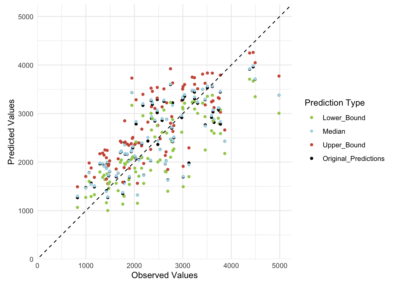
# Ensure plot_data contains 'Observed', 'Original_Predictions', 'Median', 'Lower_Bound', and 'Upper_Bound'

# Calculate summary statistics for observed values
observed_summary <- summary(plot_data$Observed)

# Calculate summary statistics for original model predictions
original_pred_summary <- summary(plot_data$Original_Predictions)

# Calculate summary statistics for bootstrap median predictions
bootstrap_median_summary <- summary(plot_data$Median)

# Create a data frame with summary statistics directly from summary objects
summary_table <- tibble(
  Statistic = c("Min.", "1st Qu.", "Median", "Mean", "3rd Qu.", "Max."),
  Observed = as.numeric(observed_summary),
  Original_Predictions = as.numeric(original_pred_summary),
  Bootstrap_Median = as.numeric(bootstrap_median_summary)
)

# Display the summary table
print(summary_table)
# A tibble: 6 × 4
Statistic Observed Original_Predictions Bootstrap_Median
<chr> <dbl> <dbl> <dbl>
1 Min. 826. 1267. 1288.
2 1st Qu. 1803. 1961. 1947.
3 Median 2398. 2413. 2431.
4 Mean 2509. 2509. 2523.
5 3rd Qu. 3104. 3206. 3217.
6 Max. 5607. 3961. 3987.PART 3
Back to Andrew Ruiz
Use the fit of model 2 using the training data you computed previously, and now use this fitted model to make predictions for the test data. This gives us an indication how our model generalizes to data that wasn’t used to construct/fit/train the model.
# Make predictions on the test dataset
test_predictions <- predict(fit_all, new_data = mav10_test_25pct)

# Assuming a regression task, extract the predicted values
# If your task is classification, adjust to use `.pred_class` or appropriate column
test_predicted_values <- test_predictions$.pred

# Optionally, compare these predicted values with the actual outcomes in your test dataset
# This step requires your test dataset to include the actual outcome variable, let's say it's named 'Y'

# Assuming the actual outcomes are in mav10_test_25pct under 'Y'
actual_outcomes <- mav10_test_25pct$Y

# Calculate performance metrics, e.g., RMSE for regression tasks
rmse_value <- sqrt(mean((actual_outcomes - test_predicted_values)^2))

# Assuming calculation of RMSE for training data is similar to test data
train_rmse <- sqrt(mean((mav10_train_75pct$Y - predict(fit_all, mav10_train_75pct)$.pred)^2))

# Create a summary table of performance metrics
performance_summary <- tibble(
  Dataset = c("Training", "Test"),
  RMSE = c(train_rmse, rmse_value)
)

# Display the table
print(performance_summary)
# A tibble: 2 × 2
Dataset RMSE
<chr> <dbl>
1 Training 627.
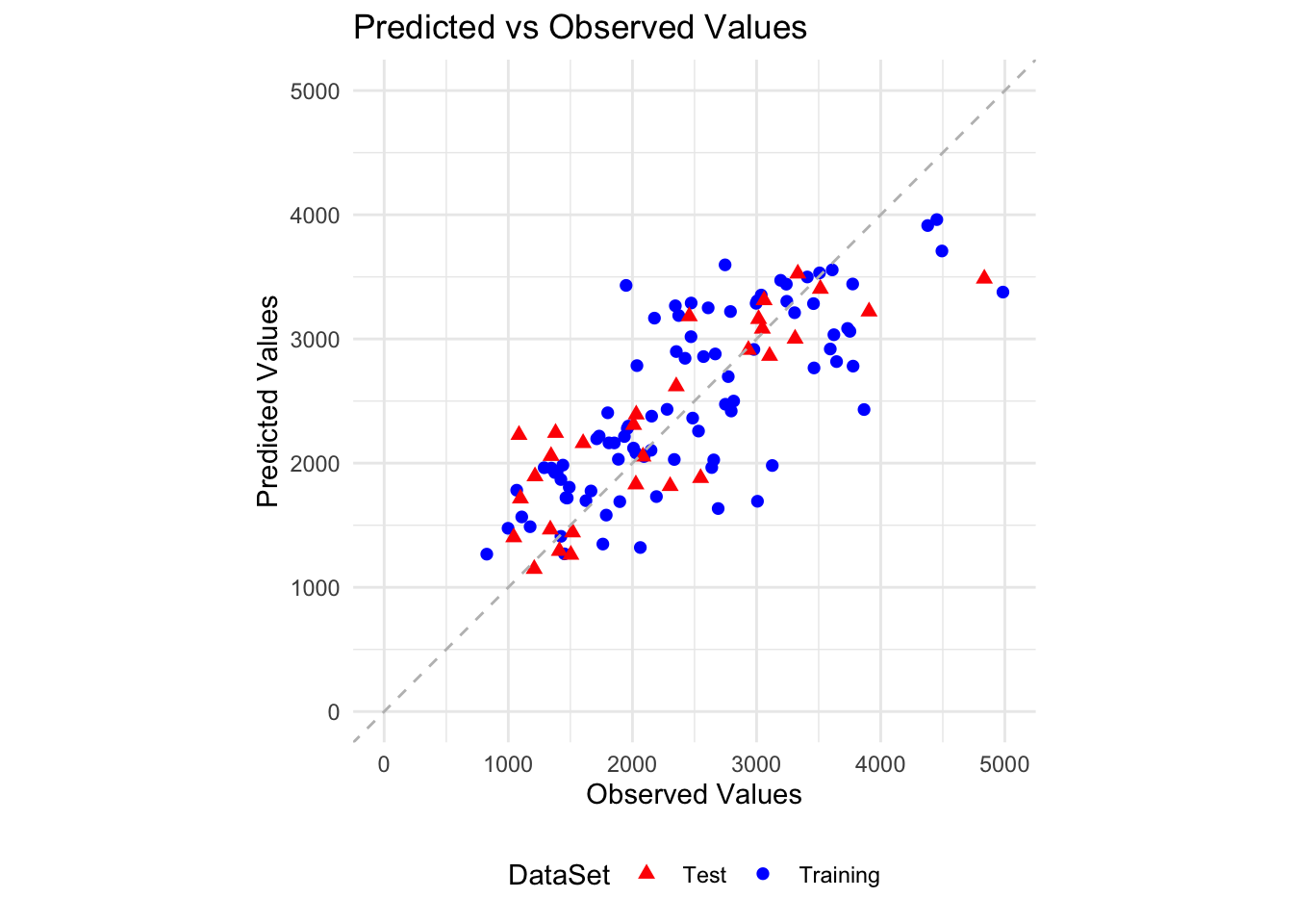
2 Test 518.Make a plot that shows predicted versus observed for both the training data (which you did above) and in the same plot, also show predicted versus observed for the test data (using, e.g. different symbols or colors).
# Step 1: Prepare the data

# For training data predictions
train_predicted_values <- predict(fit_all, new_data = mav10_train_75pct)$.pred
train_data_plot <- mav10_train_75pct %>%
  mutate(Predicted = train_predicted_values, DataSet = "Training")

# For test data predictions
test_data_plot <- mav10_test_25pct %>%
  mutate(Predicted = test_predicted_values, DataSet = "Test")

# Combine training and test data for plotting
plot_data <- bind_rows(train_data_plot, test_data_plot)

# Ensure your outcome variable name is correctly specified instead of 'Y'
plot_data$Observed <- plot_data$Y

# Step 2: Plot using ggplot2
ggplot(plot_data, aes(x = Observed, y = Predicted, color = DataSet)) +
  geom_point(aes(shape = DataSet), size = 2) +
  geom_abline(intercept = 0, slope = 1, linetype = "dashed", color = "grey") +
  scale_color_manual(values = c("Training" = "blue", "Test" = "red")) +
  labs(x = "Observed Values", y = "Predicted Values", title = "Predicted vs Observed Values") +
  theme_minimal() +
  scale_shape_manual(values = c("Training" = 16, "Test" = 17)) + # Different shapes for training and test
  xlim(0, 5000) + # Setting x-axis limits
  ylim(0, 5000) +   # Setting y-axis limits
  theme(aspect.ratio = 1, legend.position = "bottom", legend.direction = "horizontal") # Square aspect ratio and horizontal legend at the bottom
Warning: Removed 1 row containing missing values or values outside the scale range
(`geom_point()`).