cdcdata-exercise

Author

Andrew Ruiz

#Load libraries and read data

rm(list = ls())

library(here)

here() starts at /Users/andrewruiz/andrew_ruiz-MADA-portfolio

library(readr)
library(dplyr)


Attaching package: 'dplyr'

The following objects are masked from 'package:stats':

    filter, lag

The following objects are masked from 'package:base':

    intersect, setdiff, setequal, union

library(tidyr)
library(ggplot2)
library(forecast)

Registered S3 method overwritten by 'quantmod':
  method            from
  as.zoo.data.frame zoo

library(Hmisc)


Attaching package: 'Hmisc'

The following objects are masked from 'package:dplyr':

    src, summarize

The following objects are masked from 'package:base':

    format.pval, units

# Read the CSV file using here()
rabies2020 <- read_csv(here("cdcdata-exercise", "Rabies2020.csv"))

Rows: 3710 Columns: 23

── Column specification ────────────────────────────────────────────────────────
Delimiter: ","
chr (11): Reporting Area, Rabies, Animal, Current week, flag, Rabies, Animal...
dbl  (8): MMWR Year, MMWR Week, Rabies, Animal, Current week, Rabies, Animal...
lgl  (4): Rabies, Human, Current week, Rabies, Human, Previous 52 weeks Max†...

ℹ Use `spec()` to retrieve the full column specification for this data.
ℹ Specify the column types or set `show_col_types = FALSE` to quiet this message.

# Now apply your renaming and cleaning
names(rabies2020) <- gsub("[^[:alnum:] ]", "", names(rabies2020))
names(rabies2020) <- gsub(" ", "_", names(rabies2020))

rabies2020_cleaned <- rabies2020

# Check the column names
print(names(rabies2020_cleaned))

 [1] "Reporting_Area"                          
 [2] "MMWR_Year"                               
 [3] "MMWR_Week"                               
 [4] "Rabies_Animal_Current_week"              
 [5] "Rabies_Animal_Current_week_flag"         
 [6] "Rabies_Animal_Previous_52_weeks_Max"     
 [7] "Rabies_Animal_Previous_52_weeks_Max_flag"
 [8] "Rabies_Animal_Cum_2020"                  
 [9] "Rabies_Animal_Cum_2020_flag"             
[10] "Rabies_Animal_Cum_2019"                  
[11] "Rabies_Animal_Cum_2019_flag"             
[12] "Rabies_Human_Current_week"               
[13] "Rabies_Human_Current_week_flag"          
[14] "Rabies_Human_Previous_52_weeks_Max"      
[15] "Rabies_Human_Previous_52_weeks_Max_flag" 
[16] "Rabies_Human_Cum_2020"                   
[17] "Rabies_Human_Cum_2020_flag"              
[18] "Rabies_Human_Cum_2019"                   
[19] "Rabies_Human_Cum_2019_flag"              
[20] "Location_1"                              
[21] "Location_2"                              
[22] "Reporting_Area_Sort"                     
[23] "New_Georeferenced_Column"

Introduction to the data

Rabies data from the CDC

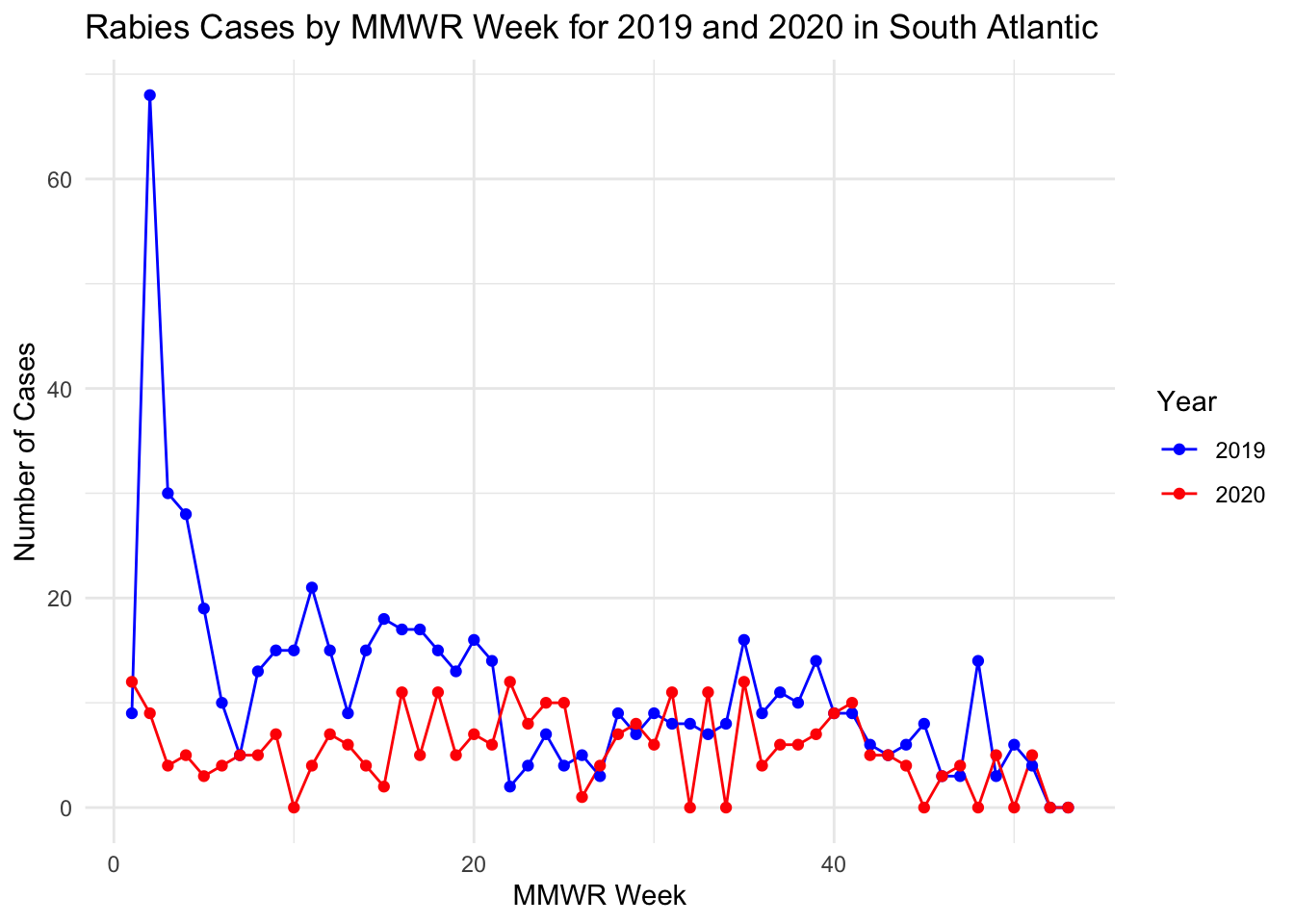
This dataset was obtained from the data.cdc.gov site link to data. It contains the count of animal and human rabies cases in the US and territories for 2020 and 2019 by MMWR Week. Since there were no human rabies cases in 2020 or 2019, this will focus on animal cases only.

Unlike human cases, which rarely go undiagnosed, animal cases are more prone to surveillance bias. Comparing the counts from 2020 to 2019, may be an important indicator of the effects of limited public health lab testing in the first year of the pandemic when public health staff were diverted to support COVID operations and some labs were closed.

Let’s look at the first few rows

head(rabies2020)

# A tibble: 6 × 23
  Reporting_Area MMWR_Year MMWR_Week Rabies_Animal_Current_week
  <chr>              <dbl>     <dbl>                      <dbl>
1 MASSACHUSETTS       2020         1                         NA
2 US RESIDENTS        2020         1                         16
3 WASHINGTON          2020         1                         NA
4 HAWAII              2020         1                         NA
5 WISCONSIN           2020         1                         NA
6 MARYLAND            2020         1                         NA
# ℹ 19 more variables: Rabies_Animal_Current_week_flag <chr>,
#   Rabies_Animal_Previous_52_weeks_Max <dbl>,
#   Rabies_Animal_Previous_52_weeks_Max_flag <chr>,
#   Rabies_Animal_Cum_2020 <dbl>, Rabies_Animal_Cum_2020_flag <chr>,
#   Rabies_Animal_Cum_2019 <dbl>, Rabies_Animal_Cum_2019_flag <chr>,
#   Rabies_Human_Current_week <lgl>, Rabies_Human_Current_week_flag <chr>,
#   Rabies_Human_Previous_52_weeks_Max <dbl>, …

print(names(rabies2020))

 [1] "Reporting_Area"                          
 [2] "MMWR_Year"                               
 [3] "MMWR_Week"                               
 [4] "Rabies_Animal_Current_week"              
 [5] "Rabies_Animal_Current_week_flag"         
 [6] "Rabies_Animal_Previous_52_weeks_Max"     
 [7] "Rabies_Animal_Previous_52_weeks_Max_flag"
 [8] "Rabies_Animal_Cum_2020"                  
 [9] "Rabies_Animal_Cum_2020_flag"             
[10] "Rabies_Animal_Cum_2019"                  
[11] "Rabies_Animal_Cum_2019_flag"             
[12] "Rabies_Human_Current_week"               
[13] "Rabies_Human_Current_week_flag"          
[14] "Rabies_Human_Previous_52_weeks_Max"      
[15] "Rabies_Human_Previous_52_weeks_Max_flag" 
[16] "Rabies_Human_Cum_2020"                   
[17] "Rabies_Human_Cum_2020_flag"              
[18] "Rabies_Human_Cum_2019"                   
[19] "Rabies_Human_Cum_2019_flag"              
[20] "Location_1"                              
[21] "Location_2"                              
[22] "Reporting_Area_Sort"                     
[23] "New_Georeferenced_Column"

Clean and process the data

# the column names have special characters that I will remove
#names(rabies2020) <- gsub("[^[:alnum:] ]", "", names(rabies2020))
#names(rabies2020) <- gsub(" ", "_", names(rabies2020))
#print(names(rabies2020))

#now select the variables we will need
rabies2020_selected <- rabies2020_cleaned %>%
  select(
    Reporting_Area, 
    MMWR_Week,      
    Rabies_Animal_Current_week,  
    Rabies_Animal_Cum_2019,      
    Location_1,    
    Location_2
  ) %>%
# Some of the count data has missing values.
# these can be replaced with zeros
# Replace NA values with 0
 mutate(
    Rabies_Animal_Current_week = replace_na(Rabies_Animal_Current_week, 0),
    Rabies_Animal_Cum_2019 = replace_na(Rabies_Animal_Cum_2019, 0)
 )
print(names(rabies2020_selected))

[1] "Reporting_Area"             "MMWR_Week"                 
[3] "Rabies_Animal_Current_week" "Rabies_Animal_Cum_2019"    
[5] "Location_1"                 "Location_2"

Now that the data is cleaner, let’s focus on the South Atlantic region for the rest of the analysis.

The original dataset does not provide the incident case count by MMWR week for 2019. Instead it only has the cumulative cases by week. We will have to create a calculate field for this so that we can make some comparisons between the years.

# Focus on South Atlantic state for the rest of the analysis
south_atlantic_data <- rabies2020_selected %>%
  filter(Location_2 == "SOUTH ATLANTIC") %>%

# Calculate incident cases for 2019
  arrange(Reporting_Area, MMWR_Week) %>%
  group_by(Reporting_Area) %>%
  mutate(Incident_Cases_2019 = Rabies_Animal_Cum_2019 - lag(Rabies_Animal_Cum_2019, default = 0)) %>%
  ungroup()
str(south_atlantic_data)

tibble [53 × 7] (S3: tbl_df/tbl/data.frame)
 $ Reporting_Area            : chr [1:53] "SOUTH ATLANTIC" "SOUTH ATLANTIC" "SOUTH ATLANTIC" "SOUTH ATLANTIC" ...
 $ MMWR_Week                 : num [1:53] 1 2 3 4 5 6 7 8 9 10 ...
 $ Rabies_Animal_Current_week: num [1:53] 12 9 4 5 3 4 5 5 7 0 ...
 $ Rabies_Animal_Cum_2019    : num [1:53] 9 77 107 135 154 164 169 182 197 212 ...
 $ Location_1                : chr [1:53] NA NA NA NA ...
 $ Location_2                : chr [1:53] "SOUTH ATLANTIC" "SOUTH ATLANTIC" "SOUTH ATLANTIC" "SOUTH ATLANTIC" ...
 $ Incident_Cases_2019       : num [1:53] 9 68 30 28 19 10 5 13 15 15 ...

Visualizing the data

Let’s create a line graph with the counts by MMWR week for both 2020 and 2019.

# Prepare data for graphing: Pivot to long format for both 2019 and 2020
south_atlantic_long <- south_atlantic_data %>%
  # Ensure MMWR_Week and Reporting_Area are retained for grouping in the long format
  pivot_longer(cols = c(Incident_Cases_2019, Rabies_Animal_Current_week), 
               names_to = "Year", 
               values_to = "Cases") %>%
  # Correct the Year column to reflect actual years
  mutate(Year = recode(Year, 
                       Incident_Cases_2019 = "2019", 
                       Rabies_Animal_Current_week = "2020"))
head(south_atlantic_long)

# A tibble: 6 × 7
  Reporting_Area MMWR_Week Rabies_Animal_Cum_2019 Location_1 Location_2    Year 
  <chr>              <dbl>                  <dbl> <chr>      <chr>         <chr>
1 SOUTH ATLANTIC         1                      9 <NA>       SOUTH ATLANT… 2019 
2 SOUTH ATLANTIC         1                      9 <NA>       SOUTH ATLANT… 2020 
3 SOUTH ATLANTIC         2                     77 <NA>       SOUTH ATLANT… 2019 
4 SOUTH ATLANTIC         2                     77 <NA>       SOUTH ATLANT… 2020 
5 SOUTH ATLANTIC         3                    107 <NA>       SOUTH ATLANT… 2019 
6 SOUTH ATLANTIC         3                    107 <NA>       SOUTH ATLANT… 2020 
# ℹ 1 more variable: Cases <dbl>

# Graph the incident animal cases from 2019 and 2020 by MMWR week
ggplot(south_atlantic_long, aes(x = MMWR_Week, y = Cases, color = Year, group = Year)) +
  geom_line() +
  geom_point() +
  theme_minimal() +
  labs(title = "Rabies Cases by MMWR Week for 2019 and 2020 in South Atlantic",
       x = "MMWR Week",
       y = "Number of Cases",
       color = "Year") +
  scale_color_manual(values = c("2019" = "blue", "2020" = "red"))

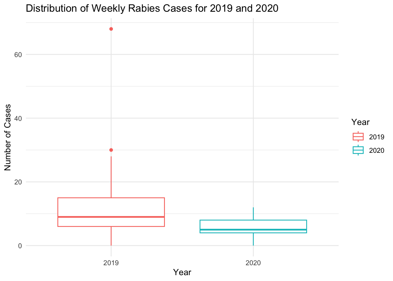
# Lets compare the two years with a box plot
ggplot(south_atlantic_long, aes(x = Year, y = Cases, color = Year)) +
  geom_boxplot() +
  theme_minimal() +
  labs(title = "Distribution of Weekly Rabies Cases for 2019 and 2020",
       x = "Year",
       y = "Number of Cases")

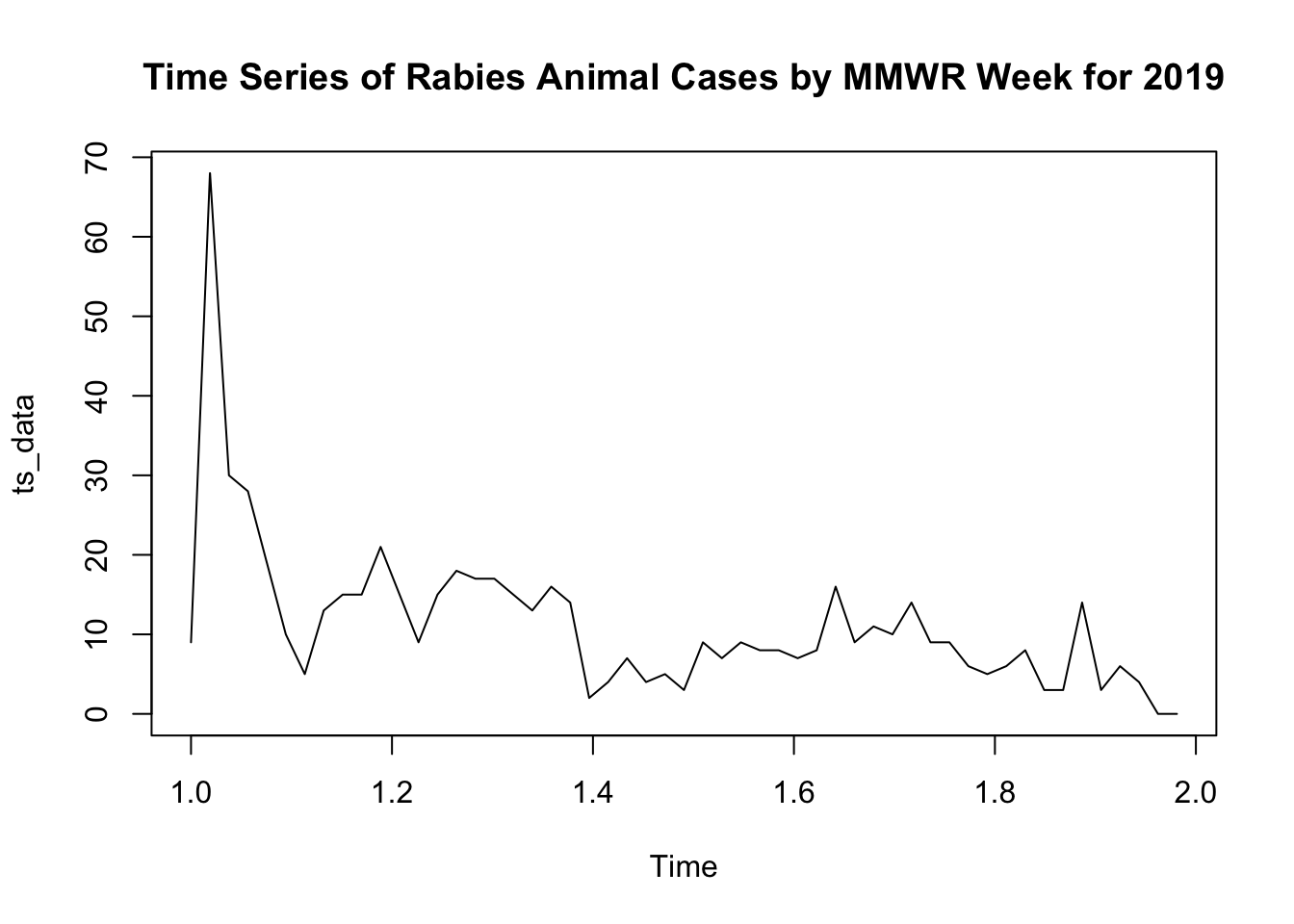
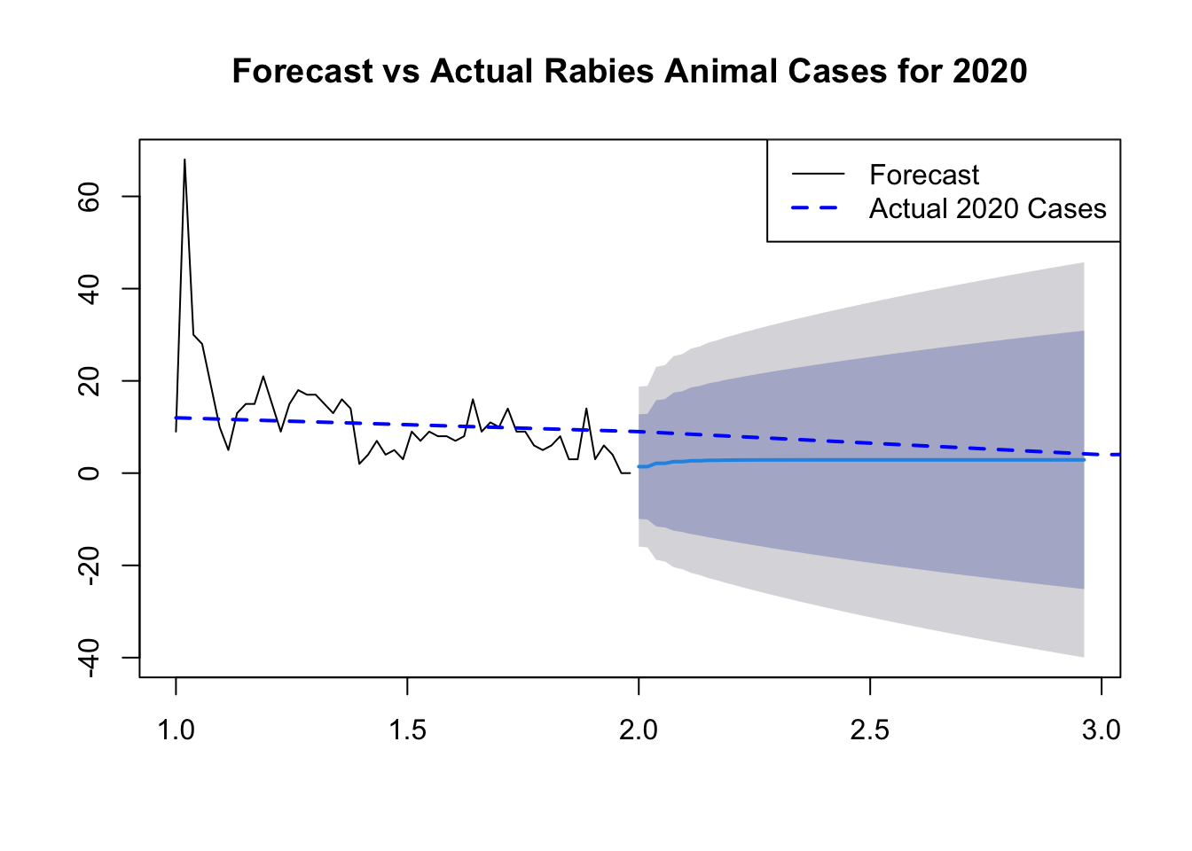
This analysis aims to understand the trends in animal rabies cases reported in the South Atlantic region during 2019, assess the model’s fit, and forecast future cases into the next year. We employ time series analysis techniques, focusing on ARIMA modeling, to capture the underlying patterns in the weekly reported cases and predict future occurrences. The process encompasses data preparation, visualization, model selection and diagnostics, and forecasting, culminating in a comparison of forecasted cases against actual data from 2020.

# Prepare the time series data
time_series_data <- south_atlantic_data %>%
  select(MMWR_Week, Incident_Cases_2019) %>%
  mutate(MMWR_Week = as.Date(paste0("2020-", MMWR_Week, "-1"), format = "%Y-%U-%u"))

Warning: There was 1 warning in `mutate()`.
ℹ In argument: `MMWR_Week = as.Date(paste0("2020-", MMWR_Week, "-1"), format =
  "%Y-%U-%u")`.
Caused by warning in `strptime()`:
! (0-based) yday 369 in year 2020 is invalid

# Convert to time series object
ts_data <- ts(time_series_data$Incident_Cases_2019, frequency = 53)

# Time Series Visualization
plot(ts_data, main = "Time Series of Rabies Animal Cases by MMWR Week for 2019")

# Modeling (Auto ARIMA)
arima_model <- auto.arima(ts_data)

# Diagnostic Checking
checkresiduals(arima_model)


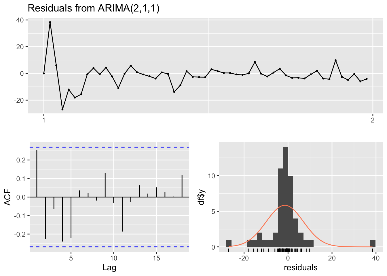
    Ljung-Box test

data:  Residuals from ARIMA(2,1,1)
Q* = 16.92, df = 8, p-value = 0.03096

Model df: 3.   Total lags used: 11

# The Ljung-Box test examined the residuals from an ARIMA(2,1,1) model 
#to see if they are correlated with each other. The test statistic (Q*) 
#was 16.92 with 8 degrees of freedom, resulting in a p-value of 0.03096. 
#This suggests that there is evidence of autocorrelation in the residuals, 
#indicating that the ARIMA model may not fully capture the underlying patterns 
#in the data.

# Forecasting
forecast_values <- forecast(arima_model, h = 52)

# Plot Forecast
#plot(forecast_values, main = "Forecast of Rabies Animal Cases for the Next 52 Weeks")

# Plot Forecast and Actual 2020 Cases
# Assuming you have the actual 2020 cases data stored in a variable called actual_2020_cases

# Plot Forecast and Actual 2020 Cases
plot(forecast_values, main = "Forecast vs Actual Rabies Animal Cases for 2020")
lines(south_atlantic_data$Rabies_Animal_Current_week, col = "blue", lty = 2, lwd = 2)  # Add actual 2020 cases to the plot

# Add legend
legend("topright", legend = c("Forecast", "Actual 2020 Cases"), col = c("black", "blue"), lty = c(1, 2), lwd = c(1, 2))

The Ljung-Box test examined the residuals from an ARIMA(2,1,1) model to see if they are correlated with each other. The test statistic (Q*) was 16.92 with 8 degrees of freedom, resulting in a p-value of 0.03096. This suggests that there is evidence of autocorrelation in the residuals, indicating that the ARIMA model may not fully capture the underlying patterns in the data.

Part 2

Contributed by Xueyan Hu

First creating a synthetic dataset

I asked AI tool google Gemini to create the codes for generating a synthetic dataset that will look like the cleaned dataset done by Andrew, but I used different names and random 2 continuous year for this synthetic dataset. It contains reporting area, the number of wwmr week in a physical year, cumulative incident of a disease (here for mine is covid) in the first year, incident cases in first year and incident cases in second year. The result was rough and wasn’t so consistant to Andrew’s original dataset, so then I asked chatGPT 3.5 to add more conditions and also by myself. The final code is as below.

# Set the seed for reproducible random numbers (optional)
set.seed(123)

# Define the number of weeks
num_weeks <- 53

# Create vectors for each variable
reporting_area <- rep("Hogwarts", num_weeks)  # All Hogwarts
mmwr_week <- rep(1:num_weeks, each = 1)  # Weeks 1 to 53

# Define the desired median
desired_median <- 6

# Generate random cases between 0-18 each week
covid_current_week <- round(
  ifelse(runif(num_weeks) < 0.01,  # 5% chance of 0
         0,
         runif(num_weeks, min = 0, max = 18)),  # Remaining 95% with range
  digits = 0
)

# Calculate the current median
current_median <- median(covid_current_week)

# Calculate the adjustment needed for the median
median_adjustment <- desired_median - current_median

# Apply the adjustment to the data
covid_current_week <- covid_current_week + median_adjustment

# Ensure all values are non-negative
covid_current_week <- pmax(covid_current_week, 0)

# Output the resulting covid_current_week vector
covid_current_week

 [1]  0  7  1  0 11 13  4  9  0  4  2 12  5 12 12 11  5 11  8 10  0  6  1  4  8
[26]  3  0  1  9  5 11  0  5 15 13 13  0  0  9  3  9  3  0 11  0  5  6  8  3  6
[51] 14  6 13

# Define the target median
target_median <- 14

# Define the fixed values and the number of weeks
fixed_values <- c(10, 70, 30)
num_fixed_weeks <- length(fixed_values)
total_weeks <- 53

# Calculate the number of fluctuating weeks
num_fluctuating_weeks <- total_weeks - num_fixed_weeks

# Calculate the sum of fixed values
fixed_sum <- sum(fixed_values)

# Calculate the target sum for the fluctuating weeks
target_sum_fluctuating <- target_median * num_fluctuating_weeks - fixed_sum

# Generate random fluctuations with the adjusted sum
fluctuations <- round(rnorm(num_fluctuating_weeks, mean = target_sum_fluctuating / num_fluctuating_weeks, sd = 5))

# Ensure all elements are non-negative
fluctuations <- pmax(fluctuations, 0)

# Combine fixed values and fluctuations
incident_case_2020 <- c(fixed_values, fluctuations)

# Enforce zeros for week 52 and 53
incident_case_2020[52:53] <- 0

# Create empty vectors for Location_1 and Location_2
location_1 <- rep(NA, num_weeks)
location_2 <- rep("Hogwarts", num_weeks)

# Set the first week to 12 and decrease to 5 on week 5
covid_current_week[1] <- 12
covid_current_week[5] <- 5

# Set last week to 0
covid_current_week[num_weeks] <- 0  

# Create the data frame
hogwarts_covid_data <- data.frame(
  Reporting_Area = reporting_area,
  MMWR_Week = mmwr_week,
  Covid_Current_Week = covid_current_week,
  Covid_Cum_2020 = cumsum(incident_case_2020),  # Cumulative cases
  Location_1 = location_1,
  Location_2 = rep("Hogwarts", num_weeks),
  Incident_Case_2020 = incident_case_2020
)

# View the data frame
print(hogwarts_covid_data)

   Reporting_Area MMWR_Week Covid_Current_Week Covid_Cum_2020 Location_1
1        Hogwarts         1                 12             10         NA
2        Hogwarts         2                  7             80         NA
3        Hogwarts         3                  1            110         NA
4        Hogwarts         4                  0            129         NA
5        Hogwarts         5                  5            140         NA
6        Hogwarts         6                 13            159         NA
7        Hogwarts         7                  4            163         NA
8        Hogwarts         8                  9            178         NA
9        Hogwarts         9                  0            190         NA
10       Hogwarts        10                  4            203         NA
11       Hogwarts        11                  2            217         NA
12       Hogwarts        12                 12            226         NA
13       Hogwarts        13                  5            236         NA
14       Hogwarts        14                 12            243         NA
15       Hogwarts        15                 12            249         NA
16       Hogwarts        16                 11            262         NA
17       Hogwarts        17                  5            276         NA
18       Hogwarts        18                 11            288         NA
19       Hogwarts        19                  8            304         NA
20       Hogwarts        20                 10            326         NA
21       Hogwarts        21                  0            335         NA
22       Hogwarts        22                  6            335         NA
23       Hogwarts        23                  1            352         NA
24       Hogwarts        24                  4            360         NA
25       Hogwarts        25                  8            368         NA
26       Hogwarts        26                  3            385         NA
27       Hogwarts        27                  0            395         NA
28       Hogwarts        28                  1            401         NA
29       Hogwarts        29                  9            414         NA
30       Hogwarts        30                  5            425         NA
31       Hogwarts        31                 11            437         NA
32       Hogwarts        32                  0            451         NA
33       Hogwarts        33                  5            461         NA
34       Hogwarts        34                 15            476         NA
35       Hogwarts        35                 13            487         NA
36       Hogwarts        36                 13            500         NA
37       Hogwarts        37                  0            517         NA
38       Hogwarts        38                  0            531         NA
39       Hogwarts        39                  9            541         NA
40       Hogwarts        40                  3            559         NA
41       Hogwarts        41                  9            576         NA
42       Hogwarts        42                  3            591         NA
43       Hogwarts        43                  0            604         NA
44       Hogwarts        44                 11            613         NA
45       Hogwarts        45                  0            632         NA
46       Hogwarts        46                  5            641         NA
47       Hogwarts        47                  6            664         NA
48       Hogwarts        48                  8            683         NA
49       Hogwarts        49                  3            694         NA
50       Hogwarts        50                  6            701         NA
51       Hogwarts        51                 14            709         NA
52       Hogwarts        52                  6            709         NA
53       Hogwarts        53                  0            709         NA
   Location_2 Incident_Case_2020
1    Hogwarts                 10
2    Hogwarts                 70
3    Hogwarts                 30
4    Hogwarts                 19
5    Hogwarts                 11
6    Hogwarts                 19
7    Hogwarts                  4
8    Hogwarts                 15
9    Hogwarts                 12
10   Hogwarts                 13
11   Hogwarts                 14
12   Hogwarts                  9
13   Hogwarts                 10
14   Hogwarts                  7
15   Hogwarts                  6
16   Hogwarts                 13
17   Hogwarts                 14
18   Hogwarts                 12
19   Hogwarts                 16
20   Hogwarts                 22
21   Hogwarts                  9
22   Hogwarts                  0
23   Hogwarts                 17
24   Hogwarts                  8
25   Hogwarts                  8
26   Hogwarts                 17
27   Hogwarts                 10
28   Hogwarts                  6
29   Hogwarts                 13
30   Hogwarts                 11
31   Hogwarts                 12
32   Hogwarts                 14
33   Hogwarts                 10
34   Hogwarts                 15
35   Hogwarts                 11
36   Hogwarts                 13
37   Hogwarts                 17
38   Hogwarts                 14
39   Hogwarts                 10
40   Hogwarts                 18
41   Hogwarts                 17
42   Hogwarts                 15
43   Hogwarts                 13
44   Hogwarts                  9
45   Hogwarts                 19
46   Hogwarts                  9
47   Hogwarts                 23
48   Hogwarts                 19
49   Hogwarts                 11
50   Hogwarts                  7
51   Hogwarts                  8
52   Hogwarts                  0
53   Hogwarts                  0

line graph for incident case by MMWR Week

# Prepare data for graphing: Pivot to long format for both 2020 and 2021
covid_data_long <- hogwarts_covid_data %>%
  pivot_longer(cols = c(Incident_Case_2020, Covid_Current_Week), 
               names_to = "Year", 
               values_to = "Cases") %>%
  # Correct the Year column to reflect actual years
  mutate(Year = recode(Year, 
                       Incident_Case_2020 = "2020", 
                       Covid_Current_Week = "2021"))
head(covid_data_long)

# A tibble: 6 × 7
  Reporting_Area MMWR_Week Covid_Cum_2020 Location_1 Location_2 Year  Cases
  <chr>              <int>          <dbl> <lgl>      <chr>      <chr> <dbl>
1 Hogwarts               1             10 NA         Hogwarts   2020     10
2 Hogwarts               1             10 NA         Hogwarts   2021     12
3 Hogwarts               2             80 NA         Hogwarts   2020     70
4 Hogwarts               2             80 NA         Hogwarts   2021      7
5 Hogwarts               3            110 NA         Hogwarts   2020     30
6 Hogwarts               3            110 NA         Hogwarts   2021      1

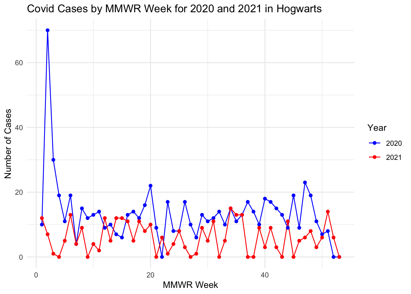
# Graph the incident animal cases from 2020 and 2021 by MMWR week
ggplot(covid_data_long, aes(x = MMWR_Week, y = Cases, color = Year, group = Year)) +
  geom_line() +
  geom_point() +
  theme_minimal() +
  labs(title = "Covid Cases by MMWR Week for 2020 and 2021 in Hogwarts",
       x = "MMWR Week",
       y = "Number of Cases",
       color = "Year") +
  scale_color_manual(values = c("2020" = "blue", "2021" = "red"))

For this line graph, I think the general trend of each year is similar with the orginal data. I noticed the feature of first year that the case number peaked at a really high point and then decreased dramatically in the several following weeks. And both first year and second year dropped to about 0 case in the last few weeks. And the average of incidence in first year is higher than second year. I tried to ask AI tool to mimic these features for me.

boxplot for incident case by year

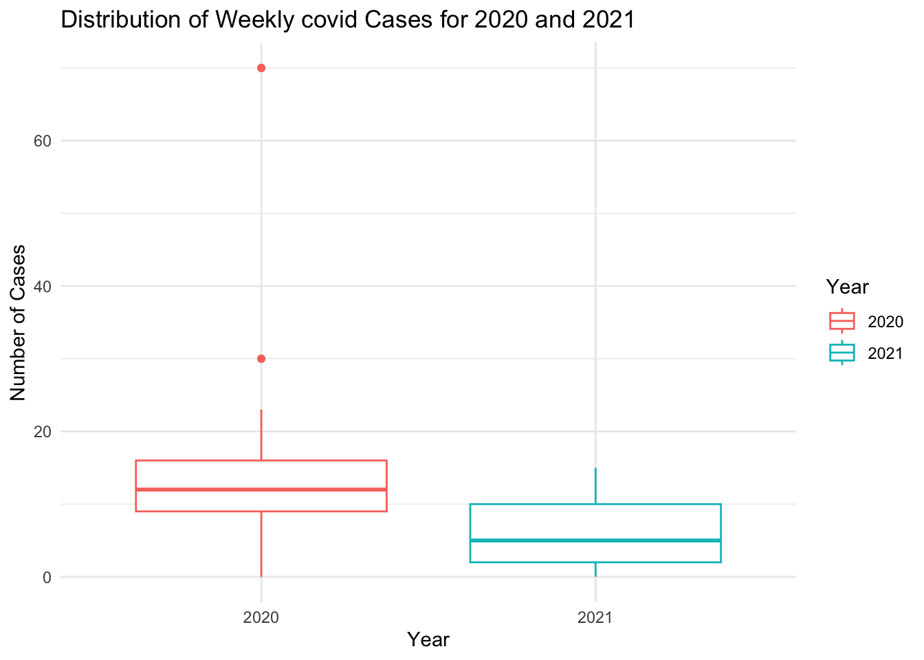
# Lets compare the two years with a box plot
ggplot(covid_data_long, aes(x = Year, y = Cases, color = Year)) +
  geom_boxplot() +
  theme_minimal() +
  labs(title = "Distribution of Weekly covid Cases for 2020 and 2021",
       x = "Year",
       y = "Number of Cases")

I think basically the boxplot has similar shape with the one generated by original data, like the medium line, out liners. But there are still some differences that I cannot eliminate. First, the 3rd quartiles and 1st quartiles are different from the original data. I have tried to ask AI tools to define the fixed values but it didn’t work well. So I only keep the right median. I couldn’t control the height of the boxes.

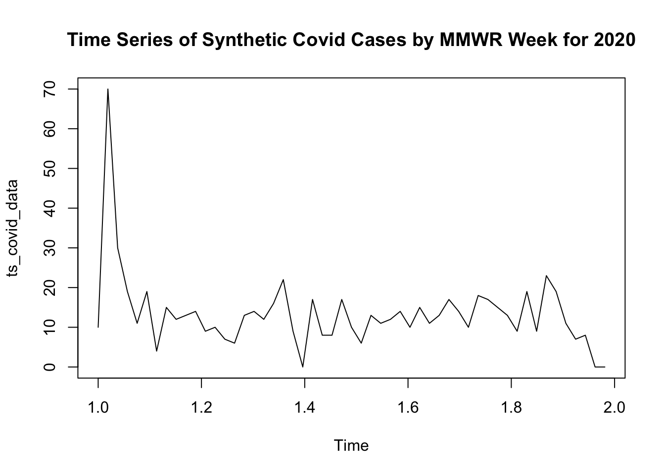
??? I don’t really know the model named ARIMA that Andrew use for doing forecasting in the last section of part 1 above. But I will copy and paste his code and run it to see what will happen here for the synthetic dataset.

# Prepare the time series data
time_series_covid_data <- hogwarts_covid_data %>%
  mutate(MMWR_Week = as.Date(paste0("2021-", MMWR_Week, "-1"), format = "%Y-%U-%u")) %>%
  select(MMWR_Week, Incident_Case_2020)

Warning: There was 1 warning in `mutate()`.
ℹ In argument: `MMWR_Week = as.Date(paste0("2021-", MMWR_Week, "-1"), format =
  "%Y-%U-%u")`.
Caused by warning in `strptime()`:
! (0-based) yday 367 in year 2021 is invalid

# Convert to time series object
ts_covid_data <- ts(time_series_covid_data$Incident_Case_2020, frequency = 53)

# Time Series Visualization
plot(ts_covid_data, main = "Time Series of Synthetic Covid Cases by MMWR Week for 2020")

# Modeling (Auto ARIMA)
covid_arima_model <- auto.arima(ts_covid_data)

# Diagnostic Checking
checkresiduals(covid_arima_model)


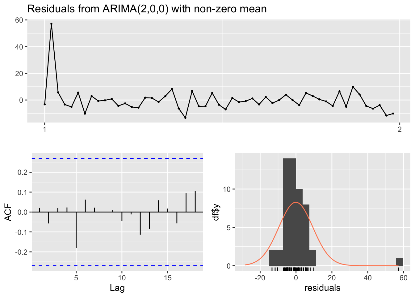
    Ljung-Box test

data:  Residuals from ARIMA(2,0,0) with non-zero mean
Q* = 2.6713, df = 9, p-value = 0.9759

Model df: 2.   Total lags used: 11

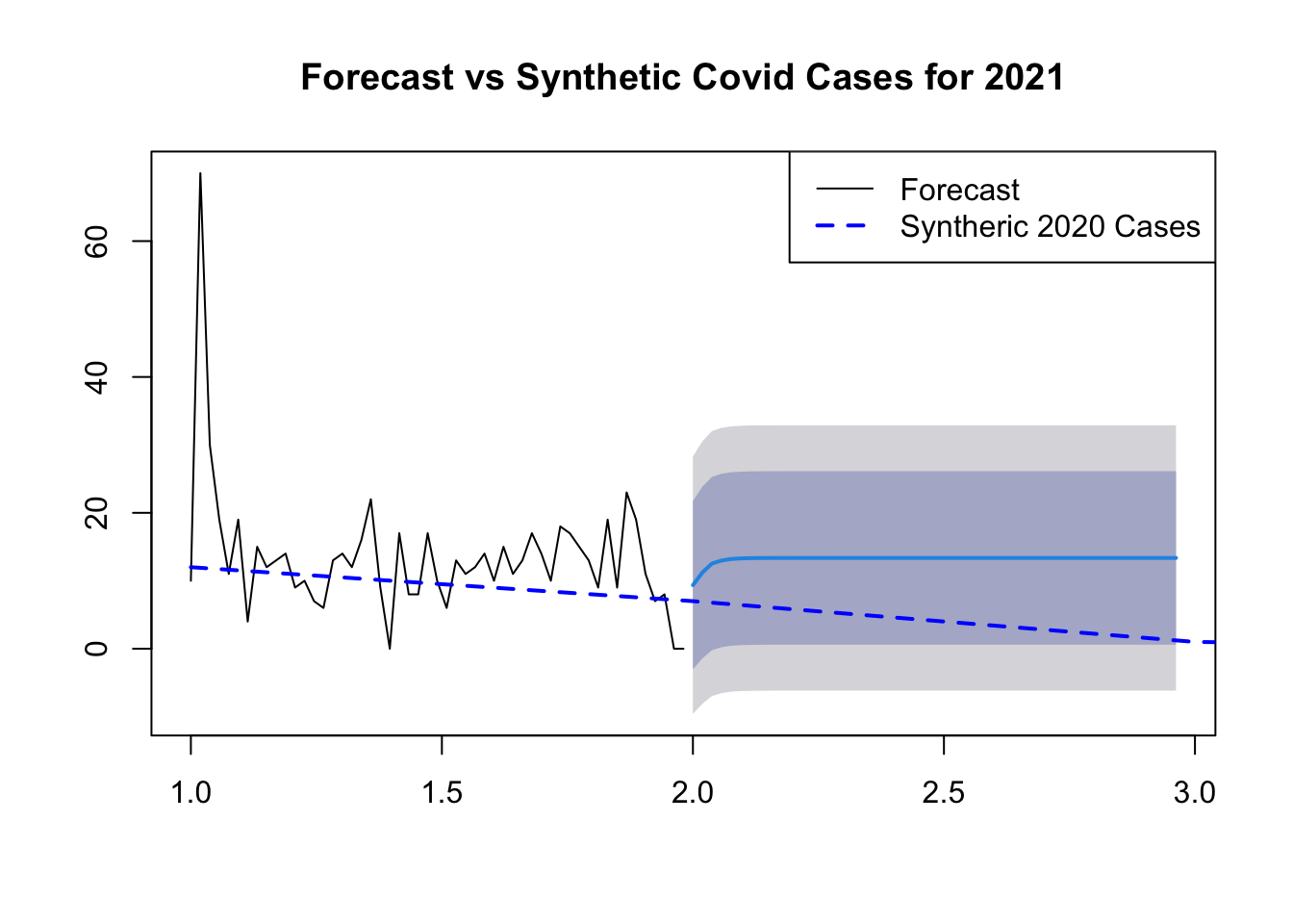
# The Ljung-Box test examined the residuals from an ARIMA(2,1,1) model 
#to see if they are correlated with each other. The test statistic (Q*) 
#was 16.92 with 8 degrees of freedom, resulting in a p-value of 0.03096. 
#This suggests that there is evidence of autocorrelation in the residuals, 
#indicating that the ARIMA model may not fully capture the underlying patterns 
#in the data.

# Forecasting
forecast_values_covid <- forecast(covid_arima_model, h = 52)

# Plot Forecast
#plot(forecast_values, main = "Forecast of Rabies Animal Cases for the Next 52 Weeks")

# Plot Forecast and Actual 2020 Cases
# Assuming you have the actual 2020 cases data stored in a variable called actual_2020_cases

# Plot Forecast and Actual 2020 Cases
plot(forecast_values_covid, main = "Forecast vs Synthetic Covid Cases for 2021")
lines(hogwarts_covid_data$Covid_Current_Week, col = "blue", lty = 2, lwd = 2)  # Add actual 2020 cases to the plot

# Add legend
legend("topright", legend = c("Forecast", "Syntheric 2020 Cases"), col = c("black", "blue"), lty = c(1, 2), lwd = c(1, 2))