Data Exercise

Analyzing text from public comments for REG 2023-02, Artificial Intelligence in Campaign Ads

Introduction:

The source of the text for this exercise come from public comments in response to Public Citizens second petition for rulemaking to the Federal Election Commission (FEC) in July, 2023. Public Citizen asked the FEC to clarify the subject of “fraudulent misrepresentation” regarding the use of AI, including deep fake technology, and open a Notice of Availability that would allow public comment.

Fifty pdfs were downloaded from the FEC site. Each pdf contained comments in response to Public Citizens petition.

These fifty documents made up the corpus for the text analysis. The process is described below.

if (!require(syuzhet)) {
  install.packages("syuzhet")
}
Loading required package: syuzhet
#load packages
library(pdftools)
Using poppler version 23.04.0
library(tm)
Loading required package: NLP
library(topicmodels)
library(syuzhet)
library(tokenizers)
library(here)
here() starts at /Users/andrewruiz/andrew_ruiz-MADA-portfolio

Process:

Locate and read the PDFs

# Specify the folder containing the PDFs
pdf_folder <- here("data-exercise", "data", "raw-data")

# Read all PDF files from the folder
file_list <- list.files(path = pdf_folder, pattern = "*.pdf", full.names = TRUE)

Process files

Now that the files are located and read, we will begin processing them for analysis

# Extract text from each PDF
text_data <- lapply(file_list, pdf_text)

# Combine the text into one character vector, one element per PDF
text_data_combined <- sapply(text_data, paste, collapse = " ")

# Create a corpus from the combined text
docs <- Corpus(VectorSource(text_data_combined))

Cleaning the text

To analyze the text we will need to clean in and prepare it for use.

clean_corpus_initial <- function(corpus) {
  original_length <- length(corpus)
  # convert text to lowercase
  corpus <- tm_map(corpus, content_transformer(tolower))
  # remove punctuation
  corpus <- tm_map(corpus, removePunctuation)
  # remove numbers
  corpus <- tm_map(corpus, removeNumbers)
  # remove stop words (common words like 'the', 'and', 'is)
  corpus <- tm_map(corpus, removeWords, stopwords("english"))
  # remove extra whitespaces
  corpus <- tm_map(corpus, stripWhitespace)
  
  # Return the cleaned corpus along with the indices of dropped documents
  return(list(corpus = corpus, original_length = original_length))
}

# Apply initial cleaning
result <- clean_corpus_initial(docs)
Warning in tm_map.SimpleCorpus(corpus, content_transformer(tolower)):
transformation drops documents
Warning in tm_map.SimpleCorpus(corpus, removePunctuation): transformation drops
documents
Warning in tm_map.SimpleCorpus(corpus, removeNumbers): transformation drops
documents
Warning in tm_map.SimpleCorpus(corpus, removeWords, stopwords("english")):
transformation drops documents
Warning in tm_map.SimpleCorpus(corpus, stripWhitespace): transformation drops
documents
# There was a warning that documents had been dropped. This code will check to see which ones and how many.
corpus_cleaned <- result$corpus
original_length <- result$original_length

cat("Original number of documents:", original_length, "\n")
Original number of documents: 50 
cat("Number of documents after cleaning:", length(corpus_cleaned), "\n")
Number of documents after cleaning: 50 
cat("Number of documents dropped:", original_length - length(corpus_cleaned), "\n")
Number of documents dropped: 0 
# Identify the indices of dropped documents
dropped_indices <- setdiff(1:original_length, 1:length(corpus_cleaned))
cat("Indices of dropped documents:", paste(dropped_indices, collapse = ", "), "\n")
Indices of dropped documents:  
# The output indicates that zero documents were dropped

Now that the text is clean we can proceed to the next step.

# Create a Document-Term Matrix (DTM) from the cleaned text documents (docs_cleaned_initial).
# Remove rows (documents) from the DTM where the sum of term frequencies is zero,
# effectively filtering out empty documents.
dtm_initial <- DocumentTermMatrix(corpus_cleaned)
dtm_initial <- dtm_initial[rowSums(as.matrix(dtm_initial)) > 0, ]

We will now create a Latent Dirichlet Allocation (LDA) model. An LDA is statistical model used in natural language processing and machine learning.

# Set the number of topics to 8
# this can be modified depending on the need and results
k_initial <- 8

# Create an LDA model using the Document-Term Matrix (dtm_initial) with the specified number of topics.
# Control parameters may include the random seed for reproducibility (seed = 4321).
lda_model_initial <- LDA(dtm_initial, k = k_initial, control = list(seed = 4321))

# Retrieve the terms associated with each topic, specifying a maximum of 8 terms per topic.
topics_initial <- terms(lda_model_initial, 8)

# Print the initial topics along with potential terms that describe each topic.
print("Initial topics with potential names included:")
[1] "Initial topics with potential names included:"
print(topics_initial)
     Topic 1        Topic 2   Topic 3      Topic 4    Topic 5     Topic 6     
[1,] "campaign"     "mary"    "campaign"   "john"     "ads"       "content"   
[2,] "comments"     "michael" "deepfakes"  "patricia" "provided"  "can"       
[3,] "ads"          "robert"  "election"   "donna"    "campaigns" "campaign"  
[4,] "deceptive"    "david"   "candidate"  "susan"    "never"     "generative"
[5,] "content"      "barbara" "political"  "linda"    "depicting" "election"  
[6,] "misleading"   "richard" "commission" "margaret" "law"       "federal"   
[7,] "saying"       "linda"   "public"     "thomas"   "comments"  "use"       
[8,] "ai‐generated" "susan"   "fraudulent" "david"    "use"       "commission"
     Topic 7      Topic 8    
[1,] "campaign"   "campaign" 
[2,] "comments"   "ads"      
[3,] "saying"     "deceptive"
[4,] "deceptive"  "law"      
[5,] "misleading" "campaigns"
[6,] "content"    "never"    
[7,] "understand" "comments" 
[8,] "release"    "depicting"

We now have 8 topics with the most common words associated with each topic. Notice that topic 2 is a list of first names. This is not especially helpful in this case. However, let’s proceed with these topics and see if we can fix them later. Next we will see the theme associated with each document.

# Extract the topic for each document for the initial model
topic_probabilities_initial <- posterior(lda_model_initial)$topics
doc_topics_initial <- apply(topic_probabilities_initial, 1, which.max)

# Create a data frame for the document-topic associations for the initial model
doc_topics_df_initial <- data.frame(Document = names(doc_topics_initial), MostLikelyTopic = doc_topics_initial)

# View the first few rows of the document-topic association for the initial model
head(doc_topics_df_initial)
  Document MostLikelyTopic
1        1               3
2        2               3
3        3               6
4        4               6
5        5               3
6        6               6

Let’s include those names in the stopword list to see if the results are better.

# Extend the stopwords list with common names for refined cleaning
custom_stopwords <- c(stopwords("en"), "john", "patricia", "donna", "susan", "linda", "margaret", "thomas", "david")

# Refined cleaning function that includes removal of first names
clean_corpus_refined <- function(corpus) {
  corpus <- tm_map(corpus, content_transformer(tolower))
  corpus <- tm_map(corpus, removePunctuation)
  corpus <- tm_map(corpus, removeNumbers)
  corpus <- tm_map(corpus, removeWords, custom_stopwords)
  corpus <- tm_map(corpus, stripWhitespace)
  return(corpus)
}
# Apply refined cleaning
docs_cleaned_refined <- clean_corpus_refined(docs)
Warning in tm_map.SimpleCorpus(corpus, content_transformer(tolower)):
transformation drops documents
Warning in tm_map.SimpleCorpus(corpus, removePunctuation): transformation drops
documents
Warning in tm_map.SimpleCorpus(corpus, removeNumbers): transformation drops
documents
Warning in tm_map.SimpleCorpus(corpus, removeWords, custom_stopwords):
transformation drops documents
Warning in tm_map.SimpleCorpus(corpus, stripWhitespace): transformation drops
documents

Now let’s rerun the code with the refined text.

# DTM for refined analysis
dtm_refined <- DocumentTermMatrix(docs_cleaned_refined)
dtm_refined <- dtm_refined[rowSums(as.matrix(dtm_refined)) > 0, ]


# Refined topic modeling
k_refined <- 8
lda_model_refined <- LDA(dtm_refined, k = k_refined, control = list(seed = 4321))
topics_refined <- terms(lda_model_refined, 8)
print("Refined topics without first names:")
[1] "Refined topics without first names:"
print(topics_refined)
     Topic 1      Topic 2      Topic 3      Topic 4   Topic 5     Topic 6    
[1,] "never"      "content"    "never"      "mary"    "ads"       "ads"      
[2,] "ads"        "election"   "ads"        "michael" "campaign"  "campaign" 
[3,] "law"        "campaign"   "comments"   "barbara" "campaigns" "never"    
[4,] "campaign"   "deepfakes"  "law"        "robert"  "deceptive" "comments" 
[5,] "misleading" "federal"    "campaign"   "nancy"   "provided"  "law"      
[6,] "americans"  "use"        "provided"   "richard" "depicting" "provided" 
[7,] "content"    "generative" "use"        "james"   "comments"  "campaigns"
[8,] "worried"    "elections"  "misleading" "carol"   "voters"    "depicting"
     Topic 7             Topic 8     
[1,] "campaign"          "campaign"  
[2,] "candidate"         "ads"       
[3,] "commission"        "fec"       
[4,] "fraudulent"        "election"  
[5,] "political"         "generative"
[6,] "deepfakes"         "federal"   
[7,] "public"            "can"       
[8,] "misrepresentation" "political" 

So it turns out that adding the names as stop words was not that helpful. It jsut returned another topic filled with names. For now, we will move on.

# Extract the topic for each document for the refined model
topic_probabilities_refined <- posterior(lda_model_refined)$topics
doc_topics_refined <- apply(topic_probabilities_refined, 1, which.max)

# Create a data frame for the document-topic associations for the refined model
doc_topics_df_refined <- data.frame(Document = names(doc_topics_refined), MostLikelyTopic = doc_topics_refined)

# View the first few rows of the document-topic association for the refined model
head(doc_topics_df_refined)
  Document MostLikelyTopic
1        1               2
2        2               2
3        3               2
4        4               2
5        5               2
6        6               2

It turns out that topic two is not associated with documents 1-6 now that names were added to the stopword list. More investigation would be needed to uncover the meaning of this. ## Sentiment analysis now let’s take a look at the sentiment for each document. For this we will use the Bing method

# Perform sentiment analysis on the combined text data
sentiment_scores <- get_sentiment(text_data_combined, method = "bing")

# View the sentiment scores
head(sentiment_scores)
[1]  -6 -24  -6  30  11  -8
# Create a vector of PDF document names
pdf_document_names <- basename(file_list)

# Create a data frame with document names and sentiment scores
sentiment_df <- data.frame(DocumentName = pdf_document_names, SentimentScore = sentiment_scores)

# Print the first few rows of the data frame to see the mapping
head(sentiment_df)
          DocumentName SentimentScore
1             aapc.pdf             -6
2 accountable_tech.pdf            -24
3              acm.pdf             -6
4            Adobe.pdf             30
5          afl_cio.pdf             11
6         arnetfox.pdf             -8
print(sentiment_df)
                           DocumentName SentimentScore
1                              aapc.pdf             -6
2                  accountable_tech.pdf            -24
3                               acm.pdf             -6
4                             Adobe.pdf             30
5                           afl_cio.pdf             11
6                          arnetfox.pdf             -8
7  AsianAmericans_advancing_justice.pdf            -16
8                       brennan_ctr.pdf             -7
9                                BS.pdf              2
10                               bv.pdf             -2
11                               ca.pdf            -72
12      campaign_for_accountability.pdf            -13
13             catholic_social_just.pdf              1
14                               cb.pdf           -131
15                     common_cause.pdf            -37
16                              CPD.pdf             -5
17                             CREW.pdf             -6
18                            crew2.pdf             -4
19               ctr_democracy_tech.pdf             -5
20            ctr_for_ai_dig_policy.pdf              0
21                               dc.pdf           -222
22                       demo_first.pdf             -3
23                              dnc.pdf            -13
24              election_protection.pdf             -2
25                             epic.pdf              4
26                     future_priva.pdf             -3
27                              GMU.pdf             -4
28                       harvardlaw.pdf            -20
29                         holtzman.pdf            -13
30 Institute for Strategic Dialogue.pdf             -5
31                   integrity_inst.pdf              1
32                        issue_dia.pdf              2
33                               jm.pdf              3
34                               lc.pdf           -241
35                              lwv.pdf              2
36                               MM.pdf              4
37                               MR.pdf            -24
38                        partnerAI.pdf              3
39              people_power_united.pdf             -4
40                              ppu.pdf              5
41                protect_democracy.pdf            -13
42                         pub_citz.pdf             -1
43                     she_persists.pdf            -21
44                      stabilityAI.pdf             21
45                        StanfordU.pdf              3
46                          technet.pdf             10
47                           unidos.pdf            -21
48                      US_congress.pdf             -1
49                            wiley.pdf            -28
50                   workers_circle.pdf             -2

For the text used in this analysis, the sentiment may be a little misleading. These comments were written in support of a second petition for the FEC to allow public comments of rulemaking. Most public comments in these forums begin by thanking the regulatory agency for allowing comments. Those sections tend to be very positive. However, the comments often continue by describing potential problem. Those tend to use negative language. The Bing method results are centered around 0. A zero score indicates completely neutral setiment. The larger negative scores indicate negative sentiment. Large positive scores indicate positive sentiment.

Let’s take a look at a different way to identify sentiment. For this we will use the NRC method which classifies sentiment into categories that may make better sense of the data.

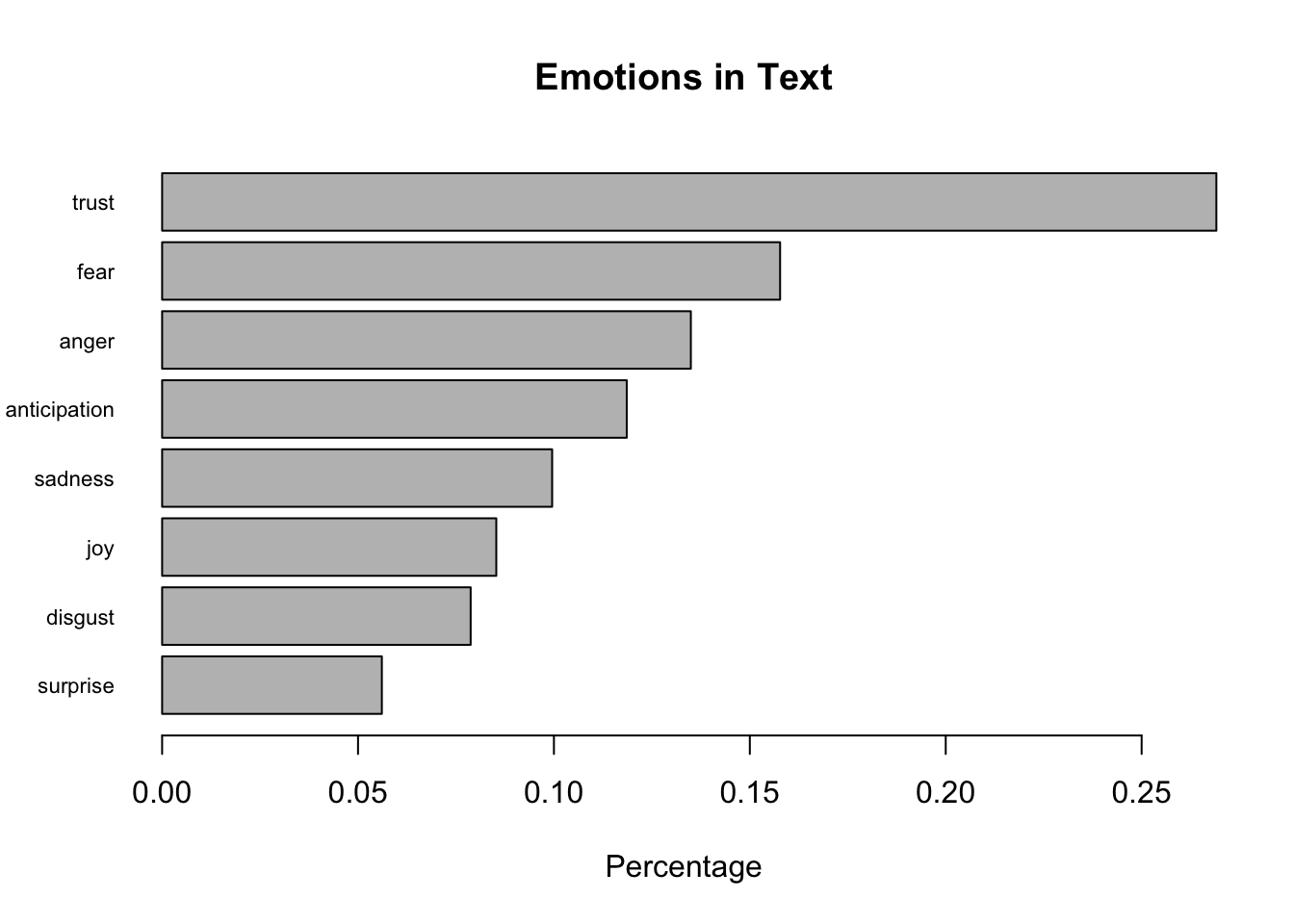
These results display word counts for the number of words in each document that fall into NRC’s sentiment categories. The bar graph represents the percent to words that fall into each category. The barchart represents all the text across all 50 documents.

# define the data
nrc_data <- get_nrc_sentiment(text_data_combined)

# Access the data frame columns for emotions and sentiments
#anger_items <- which(nrc_data$anger > 0)
#joy_items <- which(nrc_data$joy > 0)

# Print sentences associated with specific emotions
#print(text_data_combined[anger_items])
#print(text_data_combined[joy_items])

# View the entire sentiment data frame
print(nrc_data)
   anger anticipation disgust fear joy sadness surprise trust negative positive
1     10            6       6   13   5       3        4    22       21       37
2     21           13      11   22   7       6        7    28       42       24
3     11           15       7   15   8       7        5    34       26       44
4     14           24       7   20  20      13        9    51       30       92
5     16           16       7   19  12      12        7    37       29       56
6     11           11       4   12   8       4        2    27       19       43
7     17           11       6   24   6      13        4    28       34       44
8     18           18       8   16   9       7        3    34       30       50
9      1            4       1    2   2       1        1    11        8       20
10     2            0       1    3   2       0        0     2        2        4
11    68           48      39   75  29      52       27    97      133      158
12    26           19      10   25  13      17        5    53       47       72
13     6            8       3   11   7       2        5    17       15       24
14   116           86      77  134  62      97       46   163      251      263
15    31           21      15   38  15      26        9    58       66       92
16     7            8       3   13   6       3        4    23       15       30
17     9            3       6    7   3       4        2    11       16       18
18     6            5       4    9   3       2        3    19       13       23
19    18           17      10   21  13      15        7    48       46       79
20    26           42      16   37  21      22       18    89       62      132
21   161          139     100  194  93     131       79   245      374      390
22     2            4       2    3   4       3        2    10       11       19
23    17            8      12   18   5      10        7    34       35       47
24     2            2       0    4   2       0        1     3        7       10
25    11           10       5   13  14       9        6    32       30       69
26    23           20      10   23  14      12        8    48       39       80
27    19           23       8   21  22      13       10    58       48       83
28    34           33      17   36  17      18       11    61       74       94
29    20           18      13   19  10      13        7    43       51       59
30     4            2       2    3   3       4        0     9        9       15
31    24           35      11   35  19      16       11    78       57      124
32     9           11       5   15  11      12        7    40       25       51
33     2            1       2    3   5       2        0    11        7       16
34   188          124     130  213  83     168       81   229      414      357
35    12           15       5   11  10       6        5    29       20       52
36     1            1       0    1   1       0        0     4        1        4
37    17            9       8   23   7      10        2    38       44       53
38    14           22       8   16  18      10        9    53       33       74
39     3            3       2    4   3       3        1    11        8       19
40    28           30      20   28  36      21       14    46       54       96
41    21           15      12   20  12      17        6    52       49       72
42    20           21      14   18  20      19       12    65       59       91
43    16           14       8   21  12       6        5    34       35       48
44    16           27       9   21  20      10        6    56       37       92
45    10           10       6   12   6       5        0    28       22       44
46     6            9       3    8   6       3        3    25       15       42
47    19           16       8   20   7      12        5    41       35       61
48     2            2       2    5   3       1        2    13        5       23
49    15           13       8   22  13       9       11    45       44       56
50     5            3       3    4   3       3        1    10       10       17
# View only the positive and negative valence columns
print(nrc_data[, c("negative", "positive")])
   negative positive
1        21       37
2        42       24
3        26       44
4        30       92
5        29       56
6        19       43
7        34       44
8        30       50
9         8       20
10        2        4
11      133      158
12       47       72
13       15       24
14      251      263
15       66       92
16       15       30
17       16       18
18       13       23
19       46       79
20       62      132
21      374      390
22       11       19
23       35       47
24        7       10
25       30       69
26       39       80
27       48       83
28       74       94
29       51       59
30        9       15
31       57      124
32       25       51
33        7       16
34      414      357
35       20       52
36        1        4
37       44       53
38       33       74
39        8       19
40       54       96
41       49       72
42       59       91
43       35       48
44       37       92
45       22       44
46       15       42
47       35       61
48        5       23
49       44       56
50       10       17
document_sentiment <- data.frame(DocumentName = pdf_document_names, 
                                 Negative = nrc_data$negative, 
                                 Positive = nrc_data$positive)

# Print the data frame with document names and sentiment scores
print(document_sentiment)
                           DocumentName Negative Positive
1                              aapc.pdf       21       37
2                  accountable_tech.pdf       42       24
3                               acm.pdf       26       44
4                             Adobe.pdf       30       92
5                           afl_cio.pdf       29       56
6                          arnetfox.pdf       19       43
7  AsianAmericans_advancing_justice.pdf       34       44
8                       brennan_ctr.pdf       30       50
9                                BS.pdf        8       20
10                               bv.pdf        2        4
11                               ca.pdf      133      158
12      campaign_for_accountability.pdf       47       72
13             catholic_social_just.pdf       15       24
14                               cb.pdf      251      263
15                     common_cause.pdf       66       92
16                              CPD.pdf       15       30
17                             CREW.pdf       16       18
18                            crew2.pdf       13       23
19               ctr_democracy_tech.pdf       46       79
20            ctr_for_ai_dig_policy.pdf       62      132
21                               dc.pdf      374      390
22                       demo_first.pdf       11       19
23                              dnc.pdf       35       47
24              election_protection.pdf        7       10
25                             epic.pdf       30       69
26                     future_priva.pdf       39       80
27                              GMU.pdf       48       83
28                       harvardlaw.pdf       74       94
29                         holtzman.pdf       51       59
30 Institute for Strategic Dialogue.pdf        9       15
31                   integrity_inst.pdf       57      124
32                        issue_dia.pdf       25       51
33                               jm.pdf        7       16
34                               lc.pdf      414      357
35                              lwv.pdf       20       52
36                               MM.pdf        1        4
37                               MR.pdf       44       53
38                        partnerAI.pdf       33       74
39              people_power_united.pdf        8       19
40                              ppu.pdf       54       96
41                protect_democracy.pdf       49       72
42                         pub_citz.pdf       59       91
43                     she_persists.pdf       35       48
44                      stabilityAI.pdf       37       92
45                        StanfordU.pdf       22       44
46                          technet.pdf       15       42
47                           unidos.pdf       35       61
48                      US_congress.pdf        5       23
49                            wiley.pdf       44       56
50                   workers_circle.pdf       10       17
# Create a bar graph of emotions
barplot(
  sort(colSums(prop.table(nrc_data[, 1:8]))), 
  horiz = TRUE, 
  cex.names = 0.7, 
  las = 1, 
  main = "Emotions in Text", 
  xlab = "Percentage"
)